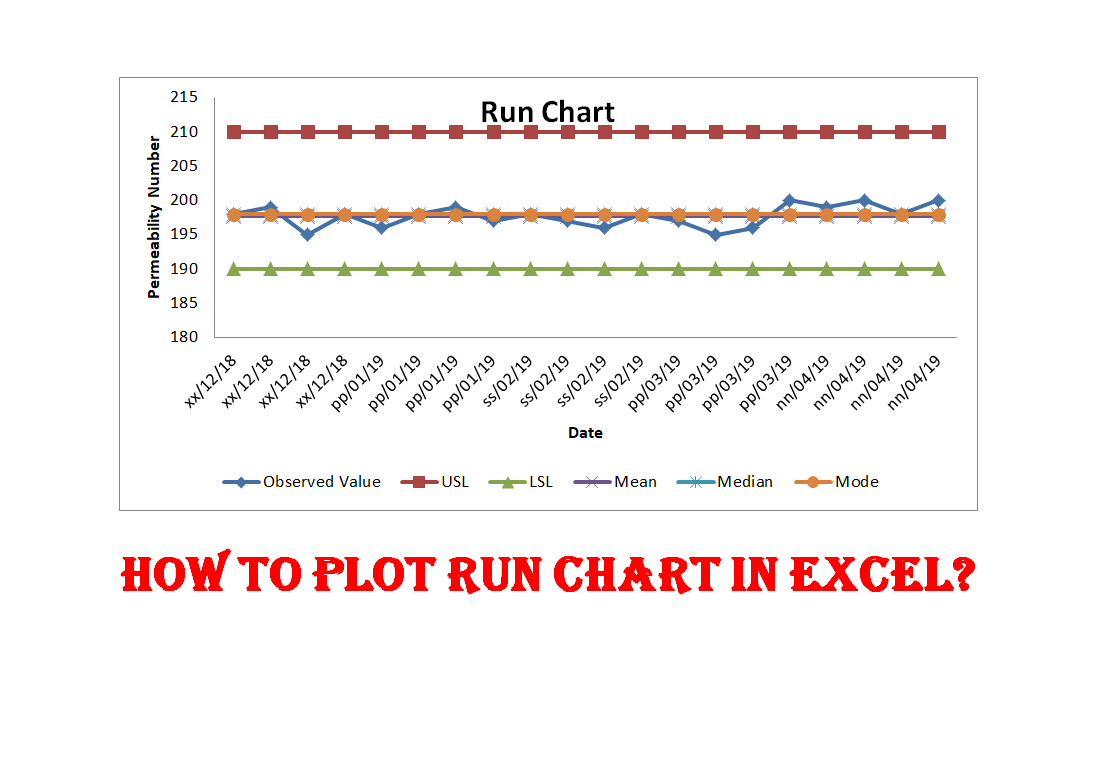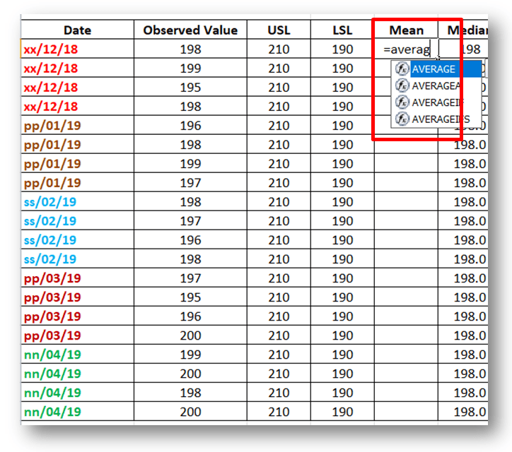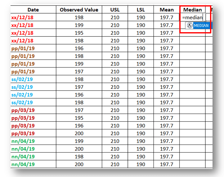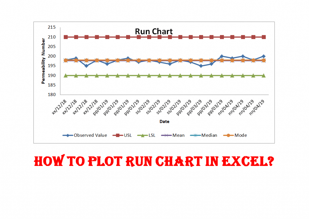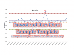
Hi Reader! Today we are going to learn how to plot a Run Chart in Minitab. A run chart is also a Line Chart. It is generally used on the shop floor to monitor the Process variation. In the run chart, you could able to set up the mean value, upper specification limit, lower specification limit, Median & mode. The Run chart will not be able to give an idea about the control limits. It represents the variation in summarizing data of Process, or Product characteristics. However, it can show you how the process is running. If you would like to download the Run Chart Excel template then click on the below link.
Step by Step guide on How to plot Run Chart in Minitab:
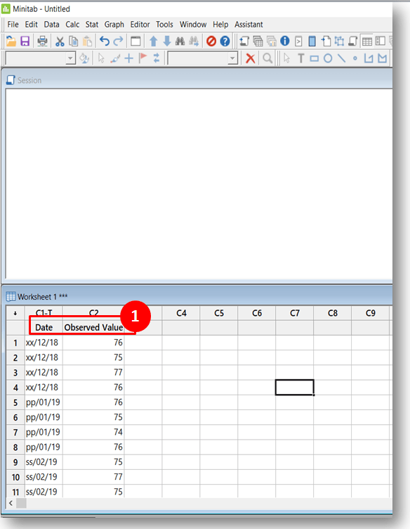
Step-1: Open the Minitab Software and enter the Reading (Observed Value).
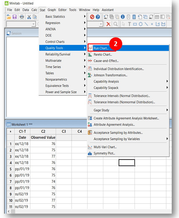
Step-2: Select the Run Chart from Minitab (Start>>Quality Tools>>Run Chart).
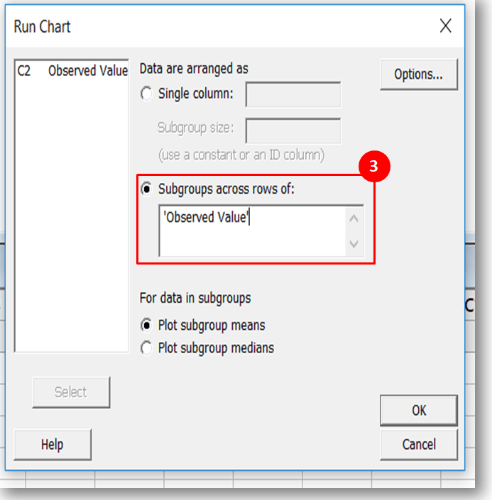
Step-3: Select the option “Subgroups across rows of”, next to click on “ok” to draw the Run Chart.
Illustration of
Steps:
Step-1:
When you will open the Minitab software; the main screen will look like below. To execute the Minitab you have to enter the data in the input sheet. Please go through the below figure to understand better.
Step-2:
Select the Run Chart option in Minitab. Go to (Start>>Quality Tools>>Run Chart).
Step-3: After selecting the “Run Chart” option in Minitab, Such below type Dialog Box will appear on the screen. Next; you have to select the Option as “Subgroups across rows of” and then finally select the Column. Look into the below figure for a better understanding.
Run Chart: –
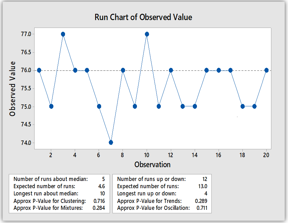
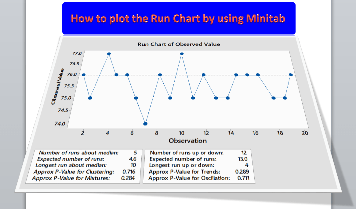
After following up the steps from Step-1 to step-3, The Run Chart will be ready to appear.
Run Chart
Interpretation of Result: A run chart will give you the approx. P-value of Clustering, Mixtures, Trends, and Oscillation. The Non-Random Variation is not available in the above Run Chart.
Shanti Gopal Pradhan is an experienced professional in Quality Management Systems, QA, Operations, Business Excellence, and Process Improvement. He has strong expertise in international standards including IATF 16949, ISO 9001, ISO 14001, ISO 45001, and ISO 17025, along with methodologies such as TQM, TPM, and Six Sigma.
He holds a degree in Mechanical Engineering along with an MBA, combining strong technical acumen with strategic business insight, he is a Certified Internal Auditor, Lead Auditor, and Six Sigma Black Belt, with a proven track record in driving quality transformation and operational excellence.
How to calculate Cp and Cpk? | Process Capability Example
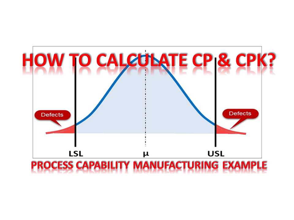
Hi readers! today we are going to discuss on Process Capability Example. The Process Capability (Cp) and Process Capability Index (Cpk) are very important tools to measure the process Capability of a Stable Process.
Process Capability Example is given below to understand better.
Process
Capability (Cp):
Process Capability (Cp) is a statistical measurement of a process’s ability to produce parts within specified limits on a consistent basis
It gives us an idea of the width of the Bell curve.
The Process Capability for a stable process is typically defined as ((USL-LSL)/ (6 x Standard Deviation)).
Process
Capability Index (Cpk):
It shows how closely a process is able to produce the output to its overall specifications.
More Value of Cpk means more process capable.
Cpk value <1 means the bell curve will be out of USL/LSL
Common Cpk vale=1,1.33,1.67 & 2
The Cpk value of a startup manufacturing organization is supposed to be 1.33.
The Process Capability Index for a stable process is typically defined as the minimum of CPU or CPL
Process Capability Example (Manufacturing Example):
The XYZ Pvt. Ltd, the organization manufactures oil sump. In their quality assurance plan, they have mentioned the Pouring Temperature (Process Parameter of the Melting Process) is a critical characteristic. So they have decided to monitor the Cp and Cpk trend.
The Specification of Pouring Temperature is
1400±10°C.
The Process Engineer has observed the Pouring Temperature and listed the same as below table;
Shanti Gopal Pradhan is an experienced professional in Quality Management Systems, QA, Operations, Business Excellence, and Process Improvement. He has strong expertise in international standards including IATF 16949, ISO 9001, ISO 14001, ISO 45001, and ISO 17025, along with methodologies such as TQM, TPM, and Six Sigma.
He holds a degree in Mechanical Engineering along with an MBA, combining strong technical acumen with strategic business insight, he is a Certified Internal Auditor, Lead Auditor, and Six Sigma Black Belt, with a proven track record in driving quality transformation and operational excellence.
Process Capability Analysis | Cp & Cpk Calculation Excel Sheet with Example
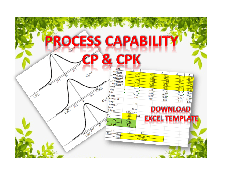
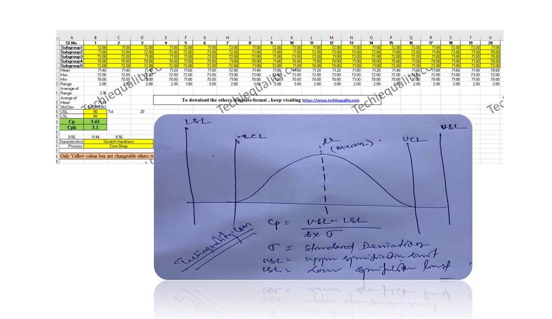
Process Capability Analysis: – The Process Capability (Cp) and Process Capability Index (Cpk) are the important tools, which give an Idea about the Process Capability of a Stable Process. Here we will discuss on Calculation of Cp and Cpk with Examples. We are offering here Process Capability Excel Template / Format for you, hence click on the below links to Download the Excel Format.
Process Capability (Cp) is a statistical measurement of a process’s ability to produce parts within specified limits on a consistent basis
It gives us an idea about the width of the Bell curve.
The Process Capability for a stable process is typically defined as ((USL-LSL)/ (6 x Standard Deviation)).
Cpk-Process Capability Index :
It shows how closely a process is able to produce the output to its overall specifications.
More Value of Cpk means more process capable.
The Process Capability Index for a stable process is typically defined as the minimum of CPU or CPL.
Process Capability Analysis:
Industrial
Example:
As per the Quality Assurance Plan, The shift engineers of Core Shop have started collecting the readings of the scratch hardness of Core. Given below are the details of Product Characteristics;
Specification of Scratch hardness is 70±10.
The Upper Specification Limit is 80.
The Lower Specification Limit is 60.
Tolerance is 20.
Scratch hardness readings Table:
Table-1
Sl.No.
1
2
3
4
5
6
7
8
9
10
SG 1
72.00
71.00
72.00
71.00
72.00
71.00
73.00
71.00
72.00
73.00
SG2
71.00
72.00
72.00
72.00
72.00
72.00
72.00
73.00
73.00
71.00
SG 3
72.00
72.00
71.00
71.00
71.00
73.00
72.00
72.00
71.00
73.00
SG4
70.00
70.00
70.00
70.00
71.00
70.00
71.00
70.00
71.00
70.00
SG 5
72.00
72.00
72.00
72.00
72.00
72.00
72.00
71.00
72.00
71.00
Table-1 [Scratch hardness readings Table]
Table-2
Sl.No.
11
12
13
14
15
16
17
18
19
20
SG1
71.00
72.00
71.00
71.00
72.00
73.00
71.00
72.00
73.00
71.00
SG2
72.00
73.00
73.00
72.00
71.00
72.00
71.00
73.00
71.00
70.00
SG3
72.00
71.00
73.00
72.00
72.00
72.00
71.00
71.00
71.00
70.00
SG4
71.00
70.00
71.00
70.00
70.00
71.00
70.00
71.00
71.00
70.00
SG5
70.00
70.00
71.00
71.00
72.00
71.00
72.00
71.00
71.00
72.00
Table-2 [Scratch hardness readings Table]
In the above two tables (Table-1 &2), we have taken the 100 readings i.e. (20 times X 5 readings at a time).
Range=Maximum Value-Minimum Value
Average of Range=2.15
Value of d2=2.326 (For Subgroup size 5)
USL = 80, LSL = 60.
Standard Deviation:
=
Average of Range/d2
2.15/2.326
=0.92
Process
Capability (Cp):
=
((USL-LSL)/ (6 x Standard Deviation))
(80-60)/ (6 x 0.92)
20/5.52
= 3.61
Process
Capability Index (Cpk):
CPU:
= ((USL-Average of Mean)/3 x Standard
Deviation)
(80-71.43)/ (3 x 0.92)
8.57/ 2.76
= 3.10
CPL:
= ((Average of Mean-LSL)/3 x Standard
Deviation)
(71.43-60)/ 2.76
10.4211.43/2.76
=4.14
Cpk= 3.10 (minimum of CPU or CPL).
After doing the Process Capability Analysis on Scratch hardness readings, we got the below result value:
Characteristics: Scratch Hardness
Cp (Process Capability) = 3.61
Cpk (Process Capability Index) = 3.10
[ Cp & CpK ]
Process Capability Analysis with Manufacturing Example
The process engineer has collected the 100 nos laddle temperature reading and the same is mentioned in the below table.
Laddle Temperature Specification= 600 ± 15°C
USL = 615
LSL = 585
Table-1
1
2
3
4
5
6
7
8
9
10
S1
605
599
610
605
603
604
600
609
605
601
S2
603
601
612
599
601
598
603
610
603
598
S3
604
598
609
610
612
609
605
612
604
603
S4
600
603
605
598
599
610
598
609
600
610
S5
602
602
607
609
605
612
599
605
609
603
Max.
605
603
612
610
612
612
605
612
609
610
Min.
600
598
605
598
599
598
598
605
600
598
Range
5
5
7
12
13
14
7
7
9
12
Average of Range
9.85
Mean
602.8
600.6
608.6
604.2
604
606.6
601
609
604.2
603
Average of Mean
603.92
Table-2
11
12
13
14
15
16
17
18
19
20
S1
599
601
602
604
598
598
609
598
600
598
S2
610
598
602
603
603
603
605
603
603
610
S3
598
603
607
598
610
607
612
607
605
598
S4
609
610
609
603
603
598
604
598
607
602
S5
600
603
605
607
598
610
603
610
598
603
Max.
610
610
609
607
610
610
612
610
607
610
Min.
598
598
602
598
598
598
603
598
598
598
Range
12
12
7
9
12
12
9
12
9
12
Mean
603.2
603
605
603
602.4
603.2
606.6
603.2
602.6
602.2
d2=2.326
Standard Deviation = Average of Range / d2 = 4.23
Cp = (USL-LSL)/6*Standard Deviation = 1.2
CPU = ((USL-Average of Mean)/3 x Standard Deviation) = 0.872
CPL = ((Average of Mean-LSL)/3 x Standard Deviation) = 1.489
CpK = 0.872(minimum of CPU or CPL).
Note: Download the Cp & Cpk excel template or format and deploy it in manufacturing process. downloading links are provided at top of this Article.
Ans.: Cp & CpK are termed as process capability and process capability index. In both cases, we would like to verify whether the process can meet the customer’s requirements or not. Generally, it is used when the process is under stable & statically control.
What is the formula of Cp & Cpk?
Cp= ((USL-LSL)/ (6 x Standard Deviation)) , where USL=Upper Specification Limit & LSL=Lower Specification Limit.
Cpk= Minimum of CPU or CPL, where CPU= ((USL-Average of Mean)/3 x Standard Deviation) & CPL= ((Average of Mean-LSL)/3 x Standard Deviation)
What are the good values of Cpk?
Generally, the customers provide the Cpk value to their supplier to maintain it in their manufacturing process. but for your knowledge, a Cpk value of 2 or greater than 2 is an excellent one.
What is cpk?
The cpk is the process capability index which shows how closely a process is able to produce the output to its overall specifications.
What is the IATF 16949 requirement of Statistical Concepts or SPC?
Application of statistical concepts in the IATF 16949 standard has been mentioned in Clause no-9.1.1.3, both Control chart (variable and Attribute) and process capability are the mandatory requirements. The application of statistical concepts shall be understood and used by the employees involved. We have published a separate article on Control Charts for our readers and you can Download Control Chart Excel Template / Format.
Shanti Gopal Pradhan is an experienced professional in Quality Management Systems, QA, Operations, Business Excellence, and Process Improvement. He has strong expertise in international standards including IATF 16949, ISO 9001, ISO 14001, ISO 45001, and ISO 17025, along with methodologies such as TQM, TPM, and Six Sigma.
He holds a degree in Mechanical Engineering along with an MBA, combining strong technical acumen with strategic business insight, he is a Certified Internal Auditor, Lead Auditor, and Six Sigma Black Belt, with a proven track record in driving quality transformation and operational excellence.
Minitab Process Capability Free Tutorial |Capability Analysis by Minitab:
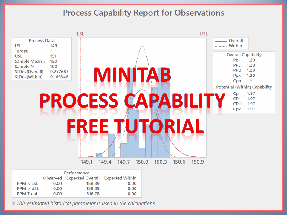
Hello! Readers, today we will guide you to learn a new topic as “how to do the Capability Analysis by Minitab18?” as you know that how process capability (Cp, Cpk) is important to know the Process consistency or Stability. To delight and enhance the customer requirement and to get the defect-free product, all critical process’s characteristics capability analysis is supposed to Monitor. Download the Minitab Process Capability free tutorial from below link.
The Customer has generally mentioned the value of Process capability and its index in CSR (Customer Specific requirement or Voice of Customer or Critical to Quality). Even after, Supplier can set their own level of Process capability index value considering with CSR and other requirements. Basically, startup company are set up the value as 1.33 at the initial stage and then to further improvement to 1.67, next 2 and onwards.
Minitab Process
Capability Tutorial (Step by Step guide):
Step-1:
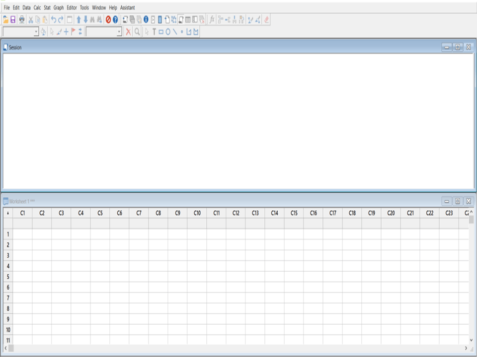
When you will open the Minitab 18, the main screen will
appear like below.
Step-2:
let’s get started with an Example, A sheet metal manufacturing company was producing Brake pad. The length of the Brake pad was 150±1mm. After stabilizing the process at “Blanking operation”, Process QC Engineer starts to analysis the Process capability and calculates the Cp & Cpk by using Minitab-18.
We would like to help my all readers to know on How to do Capability Analysis by Minitab 18?
We are having 100 numbers of data readings w.r.t below
specifications as;
Subgroup Size=5, Brake pad Length=150±1mm (LSL=149, µ=150, USL=151).
Date
Observations
12.03.2019
149.9
12.03.2019
149.3
12.03.2019
149.5
12.03.2019
149.8
12.03.2019
149.9
12.03.2019
149.8
12.03.2019
149.8
12.03.2019
149.8
12.03.2019
149.7
12.03.2019
150
12.03.2019
150.1
……
……
13.03.2019
149.5
13.03.2019
149.5
13.03.2019
149.8
13.03.2019
150.4
13.03.2019
150.4
13.03.2019
150.3
13.03.2019
150.4
13.03.2019
150.3
13.03.2019
150.3
13.03.2019
150.2
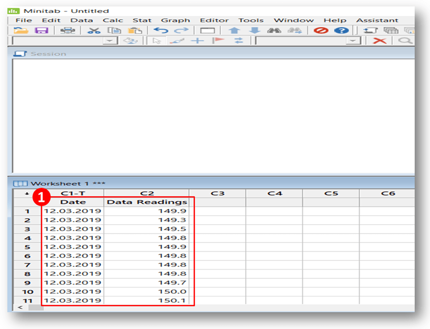
Now, you have to enter all readings in Minitab’s sheet.
Step-3:
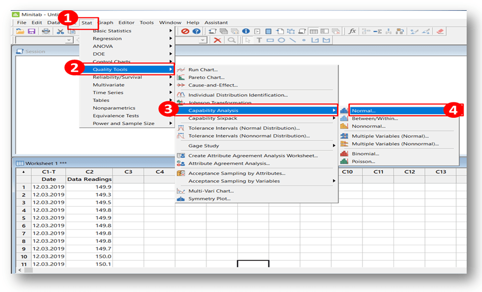
Next, you have to select the capability analysis option from Minitab’s Icon. Just follow the serial number sequence from 1 to 4 as shown in the below fire for selecting the capability analysis option.
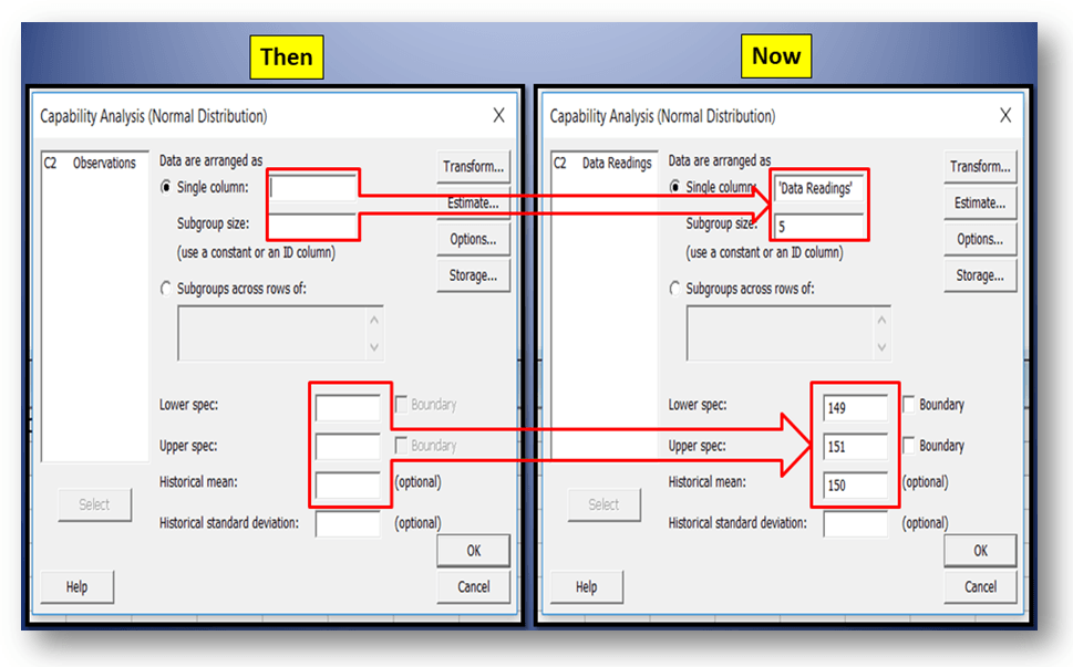
After, selecting the Capability Analysis option, a Dialog Box will appear on the screen just like below. Now, you have to set up some value in a dialog box, just go through the below figure to understand better, here we have already filled up the value w.r.t Brake pad’s specs. (Length=150±1mm, subgroup size=5). Finally, after set-up the value you are expected to click on the “ok” option in the dialog box.
Step-5:
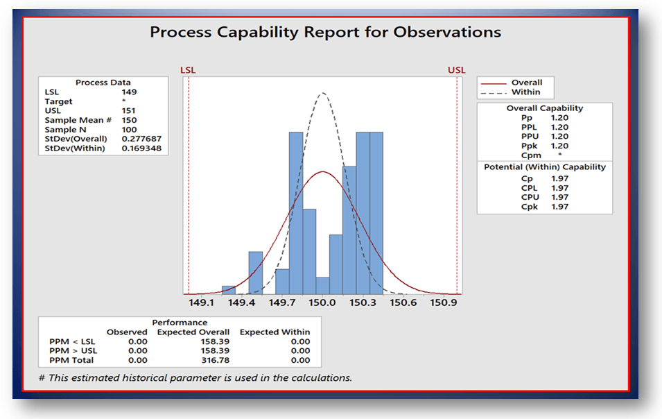
Finally, after selecting the “ok” option in the dialog box, your Process Capability value and the graph will be ready, just like below;
Shanti Gopal Pradhan is an experienced professional in Quality Management Systems, QA, Operations, Business Excellence, and Process Improvement. He has strong expertise in international standards including IATF 16949, ISO 9001, ISO 14001, ISO 45001, and ISO 17025, along with methodologies such as TQM, TPM, and Six Sigma.
He holds a degree in Mechanical Engineering along with an MBA, combining strong technical acumen with strategic business insight, he is a Certified Internal Auditor, Lead Auditor, and Six Sigma Black Belt, with a proven track record in driving quality transformation and operational excellence.
Run Chart Example | Concept & Interpretation of Result with Case Study | Industrial Example:
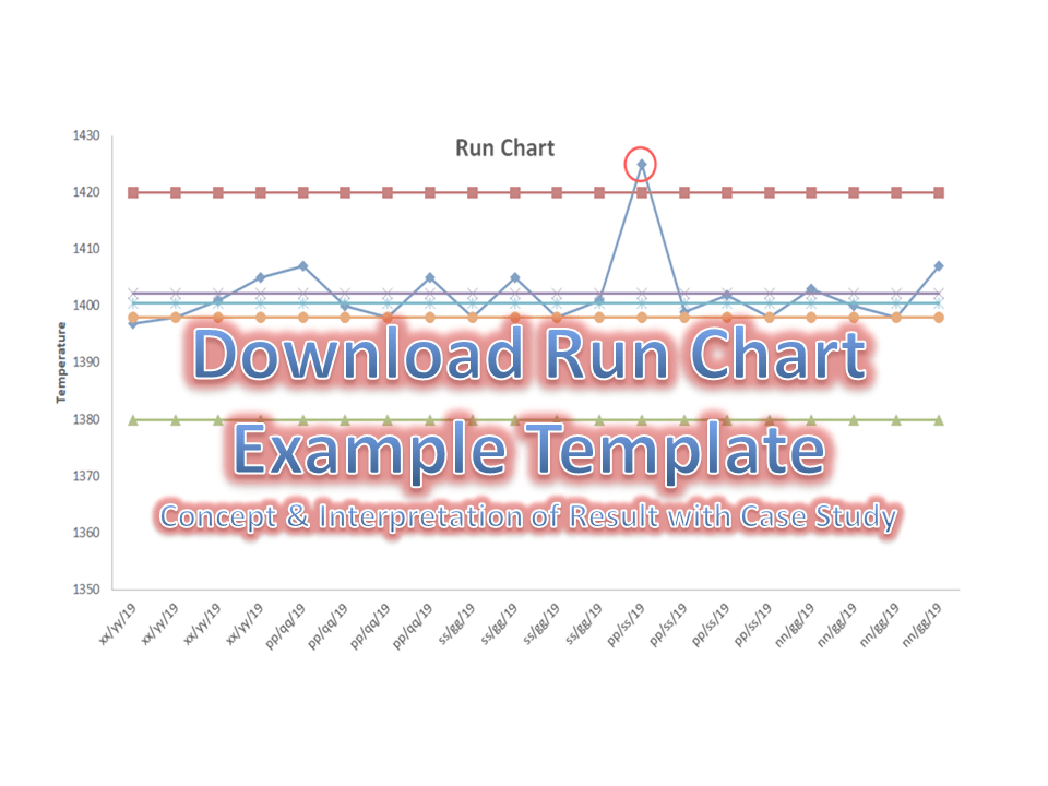
Hi readers! today we are going to discuss on Run Chart Example. A run chart is also called a Line graph. It’s a live Chart that you can use it on the shop floor to monitor the Process variation. In the run chart, you could able to set up the mean value, upper specification limit, and lower specification limit. A Run chart will not be able to give an idea about the control limits. It represents the variation in summarizing data of Process, or Product characteristics. However, it can show you how the process is running.
Interp.-1: Six or more consecutive points fall above or below the centre line (Median Line).
Interp.-2: Five or more successive points are going up or down.
Interp.-3: Too many or too few runs.
Interp.-4: An astronomical data point.
If any, one of the above interpretations has been identified in the run chart, it means variation (non-random variation) present in the process’s characteristics.
Industrial Practical Example of Run Chart (Run Chart Example):
We are going to take an example from the Iron manufacturing industry. Such a company is produced as an automobile part with the following specifications.
Pouring Temperature =1400°C±20°C.
The company has decided to maintain the variation trend of Pouring temperature. They have implemented a run chart on the shop floor to monitor and measure the variation of pouring temperature w.r.t time period. The process engineer promptly started to measure the temperature readings four times a day (three working shifts) for five days. Below are the readings for your reference as;
Temperature Reading Table:
Date
Observed Value
xx/yy/19
1397
xx/yy/19
1398
xx/yy/19
1401
xx/yy/19
1405
pp/qq/19
1407
pp/qq/19
1400
pp/qq/19
1398
pp/qq/19
1405
ss/gg/19
1398
ss/gg/19
1405
ss/gg/19
1398
ss/gg/19
1401
pp/ss/19
1425
pp/ss/19
1399
pp/ss/19
1402
pp/ss/19
1398
nn/gg/19
1403
nn/gg/19
1400
nn/gg/19
1398
nn/gg/19
1407
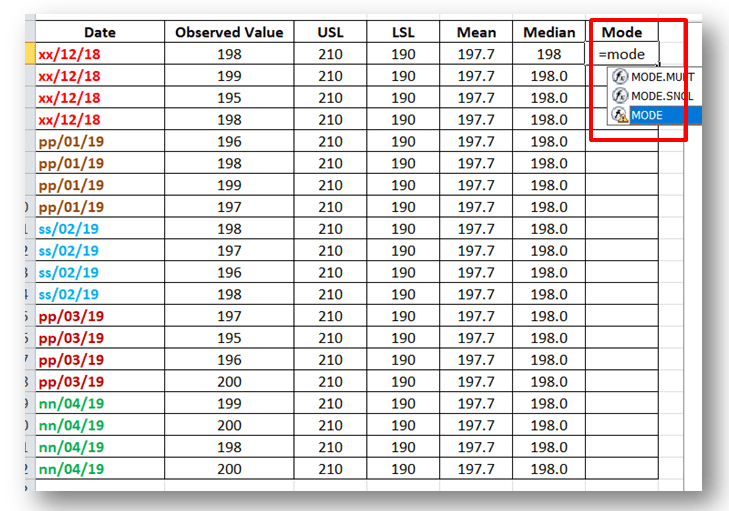
Now, we are supposed to calculate the mean, median, and mode values to plot the run chart.
Date
Observed Value
USL
LSL
Mean
Median
Mode
xx/yy/19
1397
1420
1380
1402.25
1400.5
1398
xx/yy/19
1398
1420
1380
1402.25
1400.5
1398
xx/yy/19
1401
1420
1380
1402.25
1400.5
1398
xx/yy/19
1405
1420
1380
1402.25
1400.5
1398
pp/qq/19
1407
1420
1380
1402.25
1400.5
1398
pp/qq/19
1400
1420
1380
1402.25
1400.5
1398
pp/qq/19
1398
1420
1380
1402.25
1400.5
1398
pp/qq/19
1405
1420
1380
1402.25
1400.5
1398
ss/gg/19
1398
1420
1380
1402.25
1400.5
1398
ss/gg/19
1405
1420
1380
1402.25
1400.5
1398
ss/gg/19
1398
1420
1380
1402.25
1400.5
1398
ss/gg/19
1401
1420
1380
1402.25
1400.5
1398
pp/ss/19
1425
1420
1380
1402.25
1400.5
1398
pp/ss/19
1399
1420
1380
1402.25
1400.5
1398
pp/ss/19
1402
1420
1380
1402.25
1400.5
1398
pp/ss/19
1398
1420
1380
1402.25
1400.5
1398
nn/gg/19
1403
1420
1380
1402.25
1400.5
1398
nn/gg/19
1400
1420
1380
1402.25
1400.5
1398
nn/gg/19
1398
1420
1380
1402.25
1400.5
1398
nn/gg/19
1407
1420
1380
1402.25
1400.5
1398
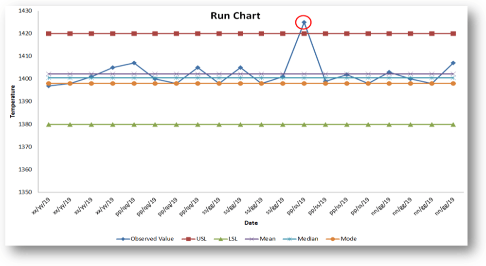
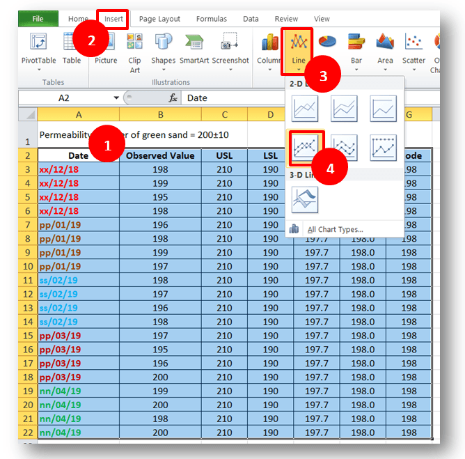
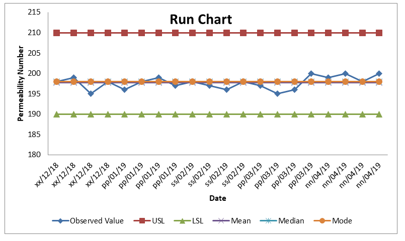
By using the aforesaid data table, we have plotted a run chart/line chart with the help of Excel. But you can also plot the run chart by Minitab such a process we will discuss later in separate articles.
Run Chart Example
[Run Chart Plot by
Excel]
Interpretation of the above run chart:
Before, we discuss the result of the above run chart. I would like to request you kindly go through the above chart prudently.
In the above chart, one reading (red highlighted point) suddenly goes up and the chart represents an astronomical data point interpretation. It means there is the existence of variation in the process and it is a non-random variation. In such a way you can plot the run chart to know how the process is running and according you could able to act on it.
Shanti Gopal Pradhan is an experienced professional in Quality Management Systems, QA, Operations, Business Excellence, and Process Improvement. He has strong expertise in international standards including IATF 16949, ISO 9001, ISO 14001, ISO 45001, and ISO 17025, along with methodologies such as TQM, TPM, and Six Sigma.
He holds a degree in Mechanical Engineering along with an MBA, combining strong technical acumen with strategic business insight, he is a Certified Internal Auditor, Lead Auditor, and Six Sigma Black Belt, with a proven track record in driving quality transformation and operational excellence.
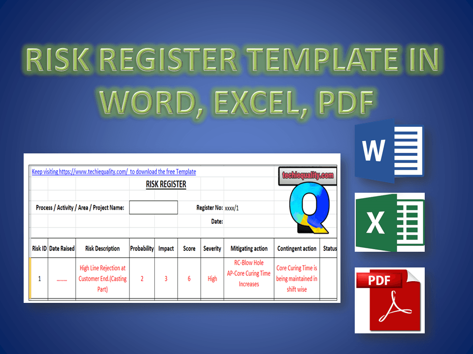
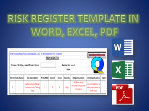
Hi Reader! Today we are going to discuss an important topic, which is called Risk-based thinking and Risk management. The organization uses different types of tools to identify the Risks but here, we will be discussing one of the popular tools, i.e. Risk Register. As we know most probably business standards like QMS, EMS, OH&SMS, etc. are now risk-based thinking approaches. So we will only concentrate on learning how to use the Risk register with Examples.
Step-1: Download the Above Template by simply clicking on the Download link.
Step-2: Read carefully the terminology.
Step-3: The severity Table is given in the Excel Template in a Separate Sheet, So don’t forget to download the Excel Template.
Step-4: Read carefully the sample example written in red colour in Template.
Example: Before I describe the Template, Please go through the below figure.
Risk Register Template
Terminology:
[1] Risk No.: Unique identification of each and every identified risk.
[2] Risk: Details about the Risk.
[3] Mitigating Action: Action to eliminate the Impact of Risk.
[4] Contingent Action: Action to eliminate the re-occurrence of Risk.
Here, in the above Figure, I have taken an Example of Customer complaints. So let’s get started with details about the above complaint.
High Line rejection at the Customer end was the Risk which has the score value 6 and severity is coming under the High Level. The criteria of probability and impact depend upon the organization’s decision. For a sample basis, I have taken the severity ranking according to the below data;
A Mitigation plan has taken w.r.t the Root Cause Analysis, so here Increasing the core curing time was thecorrective action and contingent action is thePreventive action. Which is “Core curing time is being maintained shift-wise”.
FAQ:
Q1: Where can we use this template?
A1: You can use this template in Project management, Risk Management, to identify the QMS, EMS OHSAS, and Business-related risks.
Q2: Who will decide the Criteria of Probability, Impact, and Severity?
A2: The organization itself will decide the criteria as to what it would be.
Shanti Gopal Pradhan is an experienced professional in Quality Management Systems, QA, Operations, Business Excellence, and Process Improvement. He has strong expertise in international standards including IATF 16949, ISO 9001, ISO 14001, ISO 45001, and ISO 17025, along with methodologies such as TQM, TPM, and Six Sigma.
He holds a degree in Mechanical Engineering along with an MBA, combining strong technical acumen with strategic business insight, he is a Certified Internal Auditor, Lead Auditor, and Six Sigma Black Belt, with a proven track record in driving quality transformation and operational excellence.
Control Chart Excel Template |How to Plot Control Chart in Excel | Download Template:
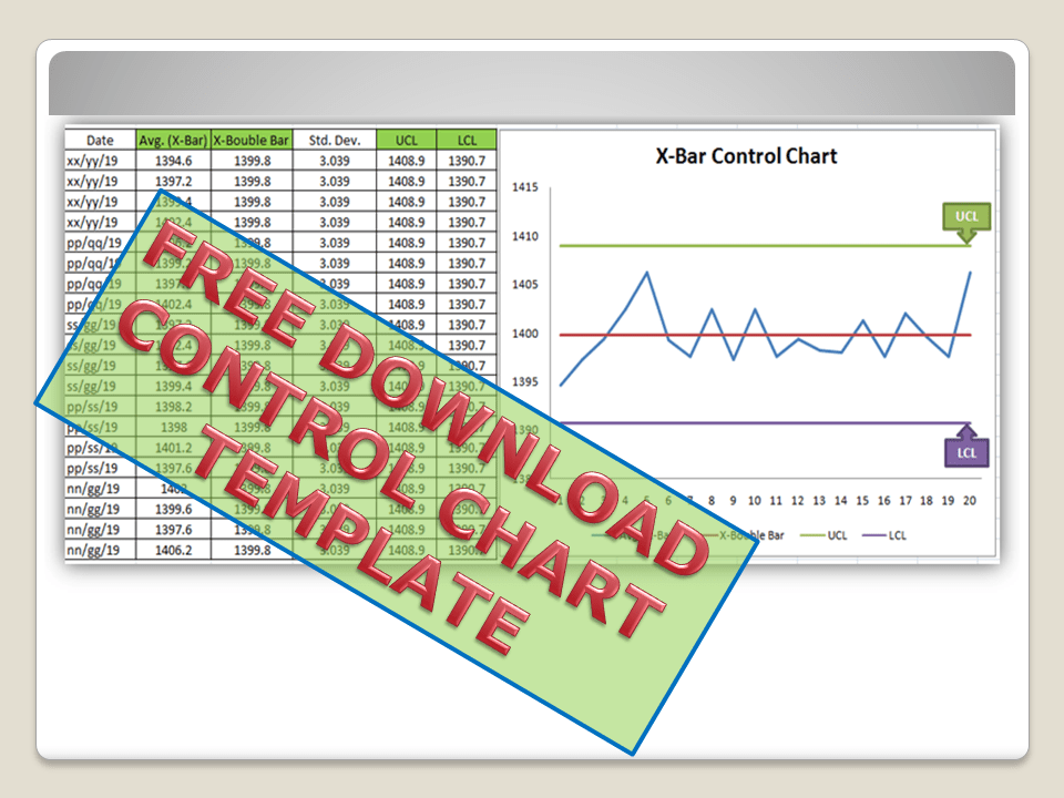
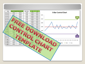
Hi! Reader, today we will guide you on how to plot a control chart in Excel with an example. To take more concentration on Process Improvement, the control chart always takes vital rules to identify the Special causes and common causes in Process Variation. Control Chart Excel Template is available here; just download it by clicking on the below link.
A Control Chart is a graphic representation of a characteristic of a process, showing plotted values of some statistic gathered from that characteristic, a centerline, and one or two control limits. It has two basic uses as an adjustment to determine if a process has been operating in statistical control and to aid in maintaining statistical control.
Control Chart Approach
for Continual Process Improvement:
Data Collection.
Control.
Analysis and Improvement.
Data Collection:-
To Collect Data and Plot the Control Chart.
Control:-
Calculate control limits from process data.
Identify Special Causes of Variation and Act upon them.
Analysis & Improvement:-
Quantify Common Cause Variation, and take action to reduce it.
How to Create Control Chart Excel Template| Step-by-Step Guides (X-Bar & Range Chart) with Example:
Step-1: Collect The Data day-wise/shift-wise.
As you can see in the above figure, we have collected data with a sample size of 5 for A-Shift with frequency (5 samples per 2 hours). So we have only one shift data for 5 days. Total 100 number observations. You are supposed to collect the data as per the Control Plan or Quality Assurance Plan.
Step-2: Select
the Data types and applicable Control Chart.
So we have variable type data and the sample size is 5. Hence the applicable Chart is the Average and Range Chart (X-Bar & Range).
Step-3: According to data type and Sample size, presently we are going to plot the X-Bar & R-Chart. So individually we will plot both charts (X-Bar Chart & Range Chart). First, we will plot the X-bar chart and then the R-chart.
3.1 X-Bar Chart:
Before we start, just go through the green highlighted terms in the above figure as [1] Average
[2] X-Double Bar means an average of average. [3] Standard Deviation. [4] UCL. [5] LCL.
Calculation:
[1] Average:
Make sure that your attention is now on the right side corner of the above figure. To calculate the average value of individual subgroup size. You have to type as (=average)and then double click on the average function and next select the sample value from x1 to x5.
[2] X-Double Bar: After calculating the Average value of all Subgroups (Individual Date wise), now we have to calculate the average of Average (Average of X-Bar).
[3] Standard
Deviation: Standard Deviation of Average (X-Bar),
Type as (=Stdev) and select all X-Bar Data to Calculate the
Std. Dev. of Average.
[4] UCL:
UCL=X Double Bar +3*Sigma
UCL= X Double Bar +3*Standard Deviation
For the calculation of the UCL in Excel use the above formula.
[5]LCL:
LCL=X Double Bar -3*Sigma
LCL= X Double Bar -3*Standard Deviation
Use the above Formula in Excel.
3.11 Plot X-Bar Chart: This is the last step to plot the X-Bar Chart by using Line Graph in Excel, follow the below steps:
Simply Follow Sl. No.1 to 4.
In Sl. No.1, Select X-Bar, X-Double Bar, UCL, LCL, and then select Insert Option and next to Line Chart. After selecting the Line Graph/Chart, The X-Bar Control Chart Excel Template will be ready as below.
3.2 Range Chart:
To Plot the
R-Control Chart, we have to calculate the [1] Range. [2] R-Bar (Average of
Range). [3]UCL. [4]LCL.
[1] Range: R=Max. Value – Min. Value of Subgroup.
[2] R- Bar (Average of Range): Put the Excel formula of average.
[3] UCL:
UCL= D4 x R-Bar
UCL= 2.114 x R-Bar Value of individual Subgroup. (Note for
Subgroup Size 5, D4=2.114).
Use this formula in Excel to calculate the UCL.
[4] LCL:
LCL=D3 x R-Bar
LCL=0 (Note Foe subgroup size 5, D3=0)
Simply put the “0” in the Excel sheet.
3.22 Plot R-Chart: Just follow steps 1 to 3, and select the line chart.
In step-1, you have to select the “Range, R-Bar, UCL, and
LCL” simultaneously and then select the Line Chart, after selecting the line
chart R-Control Chart Excel Template will be ready as below
Q2: How to add upper and lower control limits in Excel?
A2: Carefully read the aforesaid Articles.
Q3: How to create a control chart in Excel 2013?
A3: Step by Step guide is described above with Statistical process control chart examples. Please go through it.
Q4: How to create a Six Sigma control chart in Excel?
A4: Control charts are classified into two types [1] Variable type and [2] Attribute Type. Both two types are further classified into several as
[1]Variable types
X and MR Chart
X-Bar and Range
X-Bar and S
[2] Attribute Chart
np-chart
p-chart
u-chart
c-chart
In the above articles, we have described only how to create an X-bar and range type Control Chart in Excel with a process control chart example. As you can see all these above types of control charts are used in Six Sigma projects but the applicable chart depends on Data type and Subgroup size (Sample size).
Q5: How to calculate upper and lower control limits (UCL & LCL) in Excel?
A5: For X-Bar
Chart-UCL:
UCL=X Double Bar +3*Sigma
UCL= X Double Bar +3*Standard Deviation
For the calculation of the UCL in Excel, use the above formula.
LCL:
LCL=X Double Bar -3*Sigma
LCL= X Double Bar -3*Standard Deviation
Use the above Formula in Excel.
For R-Chart:
UCL:
UCL= D4 x R-Bar
UCL= 2.114 x R-Bar Value of individual Subgroup. (Note for
Subgroup Size 5, D4=2.114).
Shanti Gopal Pradhan is an experienced professional in Quality Management Systems, QA, Operations, Business Excellence, and Process Improvement. He has strong expertise in international standards including IATF 16949, ISO 9001, ISO 14001, ISO 45001, and ISO 17025, along with methodologies such as TQM, TPM, and Six Sigma.
He holds a degree in Mechanical Engineering along with an MBA, combining strong technical acumen with strategic business insight, he is a Certified Internal Auditor, Lead Auditor, and Six Sigma Black Belt, with a proven track record in driving quality transformation and operational excellence.
How to fill up 8D Report Template |8D Report Example:
Hi. ! Reader, today we will discuss the 8D Report Example, case study, and How to fill up the 8D Report Template, if you have not yet downloaded the 8D Template then download the Format /template /form by clicking on the below link.
8D Report Example | Step-by-Step Guides: Example-1: There is a Customer Complaint i.e. Shrinkage on the Sump (Automobile casting part). And we have done the case study of said customer complaint and filled up the 8D template. Details are illustrated below
D1- SUPPLIER TEAM MEMBER NAMES: Champion name, Team Leader name, and Team Member name.
D2- PROBLEM DESCRIPTION e.g. Shrinkage Defect.
What
Shrinkage
Who
Customer name
Where
In Process
When
Last batch
Why
SH in Ingate
How Much
2%
D-2 (5W1H Form)
D3- IMPLEMENTING CONTAINMENT ACTION:
Target date
Actual date
Immediate stop the consignment & segregate good parts
2.2.19
2.2.19
D-3-Containment Action Table
D4- IDENTIFY PROBLEM ROOT CAUSE:
Why1
Why SH at Ingate area
Why2
Why high pouring temperature
Why3
Why pyrometer reading was not correct
Why4
Why checking of pyrometer’s condition was not done
Why5
Why-Why Analysis
Root Cause
Checking of pyrometer’s condition was not done
D-4
D5- PERMANENT CORRECTIVE ACTIONS:
Corrective Action Plan
Resp. by
PM/ Condition of Pyrometer will be checked periodically w.r.t Master one.
Maintenance Supervisor
D-5-CAP
D6- IMPLEMENT PERMANENT CORRECTIVE ACTIONS:
Corrective Action Plan
Resp. by
Target date
The actual date of Completion
A weekly PM/Condition checking Schedule has been made and checked all Pyrometer
Maintenance Supervisor
10.02.2019
10.02.2019
D-6
D7- PREVENT RECURRENCE:
Preventive Action Plan
Resp. by
Target date
The actual date of Completion
A weekly schedule will be made
Maintenance Supervisor
Weekly
Continuing
D-7-PR
D8- TEAM AND INDIVIDUAL RECOGNITION: Congratulations to the team member.
In the first case study, we have discussed in ingate shrinkage of the sump and filled up all the analysis in 8D-Template, and now, we are going to discuss another case study i.e. CS No-2, details of the analysis are illustrated below.
Case Study 2: Pin-hole Defects (Casting)
A Company PQR Ltd found nearly 3% of the last batch of BOP items as defective after machining operation due to a pinhole defect in casting. So the purchase head decided to ask and submit the full analysis of the said problem to their supplier in the 8D report. The same Analysis is illustrated below.
D1- SUPPLIER TEAM MEMBER NAMES: Champion name, Team Leader name, and Team Member name.
D2- PROBLEM DESCRIPTION e.g. Pin-hole Defect.
What
Pin-hole
Who
M/S PQR Ltd
Where
In-process
When
Last batch
Why
Pin-hole at casting base
How much
3%
5W1H
D3- IMPLEMENTING CONTAINMENT ACTION:
ICA
Segregate the defective part (pin-hole defect)
Containment Action
D4- IDENTIFY PROBLEM ROOT CAUSE:
Why-1
Why pin-hole?
Why-2
Why the core problem?
Why-3
Why core was not cured properly?
Why-4
Why the curing/drying time was not modified?
Why-5
5W Analysis
Root Cause
Curing/drying time was not validated
RC
D5- PERMANENT CORRECTIVE ACTIONS:
Corrective action plan
Resp. by
Process and product will validate w.r.t new drying time
Process QA Engineer
CA
D6- IMPLEMENT PERMANENT CORRECTIVE ACTIONS:
Corrective action plan
Resp. by
Target date
Actual Date
10 samples will be made & respective process & product characteristics will be checked whether the characteristics are meeting the specifications or not.
Process QA Engineer
xx/yy/2020
xx/yy/2020
IPCR
D7- PREVENT RECURRENCE:
Preventive action plan
Resp. by
Target Date
Actual Date
Validation process SOP will be made including change control
QA.Engineer
xx/yy/2020
xx/yy/2020
PR
D8- TEAM AND INDIVIDUAL RECOGNITION: Congratulations to the team member.
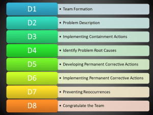
The 8D is eight disciplines of problem-solving, these are mainly, 1-supplier team member names, 2-problem description, 3-implementing containment action, 4-identify problem root cause, 5-permanent corrective actions, 6-implement permanent corrective actions, 7-prevent recurrence, 8-team, and individual recognition.
What are the 8 disciplines of an 8D-DMN report?
The 8D has 8 nos disciplines which makes it a systematic way to resolve the problem and the disciplines are
Team Formation or Establishing the team or creating a team.
Problem Description or defining the problem.
Implementing containment actions or Interim action.
Identify the problem’s root cause or RCA.
Developing permanent corrective actions or corrective action
Implementing permanent corrective actions or implementing & validating corrective actions
Preventing reoccurrences or preventive actions
Congratulate the team or Team & individual recognition.
The 8D-DMN is a very popular methodology that is frequently used in manufacturing industries to resolve the notified defective material in all the stages including customer complaints as well. we have already discussed two no case studies or practical manufacturing examples for a better understanding of the concept, application, and thorough knowledge of 8D template or format.
This concept enhances your depth of knowledge on 8D and its principles on how to fill up the template or format, which is described above. After doing so your confidence in 8D activities for internal application and for application on customer complaints will be enhanced.
Shanti Gopal Pradhan is an experienced professional in Quality Management Systems, QA, Operations, Business Excellence, and Process Improvement. He has strong expertise in international standards including IATF 16949, ISO 9001, ISO 14001, ISO 45001, and ISO 17025, along with methodologies such as TQM, TPM, and Six Sigma.
He holds a degree in Mechanical Engineering along with an MBA, combining strong technical acumen with strategic business insight, he is a Certified Internal Auditor, Lead Auditor, and Six Sigma Black Belt, with a proven track record in driving quality transformation and operational excellence.
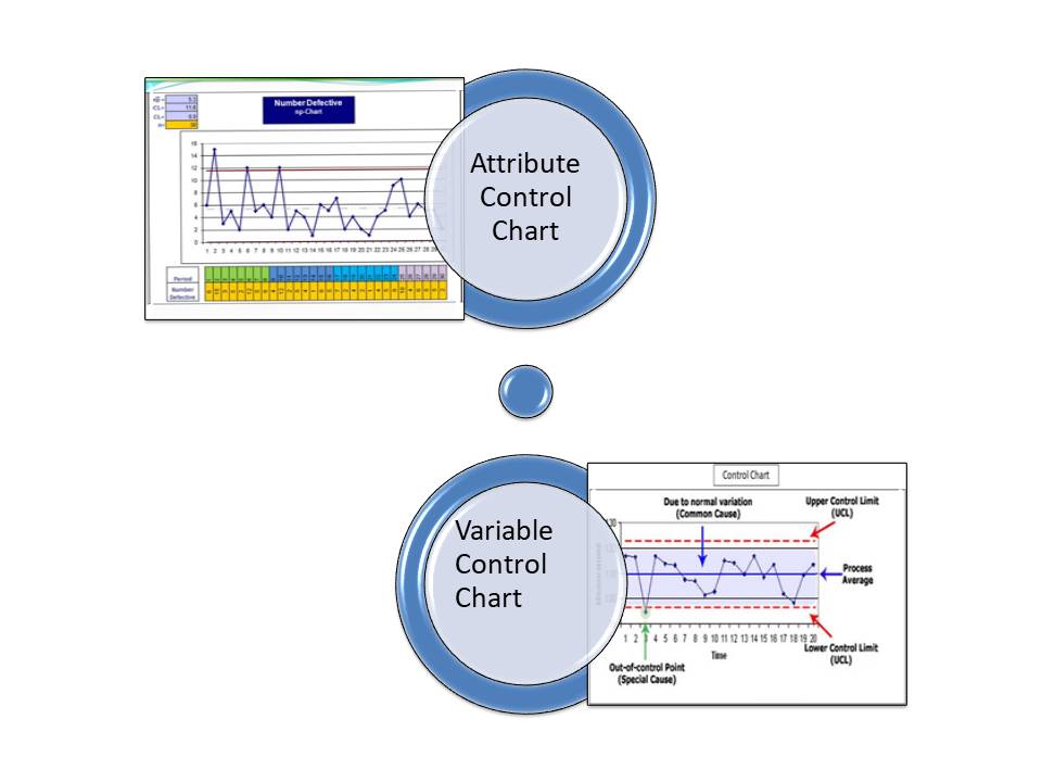
A control Chart is a popular tool to identify the process Variations and causes (Common or Special Cause). If you would like to know more about different types of Control Charts then read “What is SPC?”. You will also like to read on “how to plot a control chart in Excel’.
Steps of how to Create Control Chart in Minitab 18:
Step-1:
When you will open the Minitab 18, the main screen will appear like below.
Step-2:
Let’s take an example here to understand better. We are having 100
numbers reading of a block’s length as,
Length of Block=120±1mm, Subgroup Size=5, Sample frequency=5 samples per hour.
Date
Observations/Reading
12.03.2019
119.5
12.03.2019
119.3
12.03.2019
119.4
12.03.2019
119.5
12.03.2019
119.7
12.03.2019
120
12.03.2019
120.1
12.03.2019
120.5
12.03.2019
120.3
12.03.2019
120.4
12.03.2019
120.4
12.03.2019
120.6
12.03.2019
120.3
12.03.2019
119.7
12.03.2019
119.8
12.03.2019
119.2
12.03.2019
119.5
…..
….
13.03.2019
121.1
13.03.2019
120.2
13.03.2019
120.3
13.03.2019
120.4
13.03.2019
120.5
13.03.2019
120.9
13.03.2019
120.8
13.03.2019
120
13.03.2019
120.1
As you can see in the above figure, the same 100-number reading has been entered in box no.1. Now we are supposed to select the Average and range type Chart (because length readings are variable data and we have taken subgroup size is 5). If you would like to know the selection process of different types of Control Charts then read the article “What is SPC?”. Just follow the step-2 to step-5 in the above figure to select the “Average & Range” type control chart.
Step-3:
After selecting the “X-bar & Range chart”, such a dialog box will appear on the screen. Now just give more focus on below dialog box, because I will be describing it one by one here. In the box no-1, you can able to see the data point’s column. Now you have to select the data point in box no-3, and then enter “5” in box-4. Next, we have to enter labels to write the Title name.
Step-4:
Title name
1. Enter on Labels.
2. Name the title as you wish.
Step-5
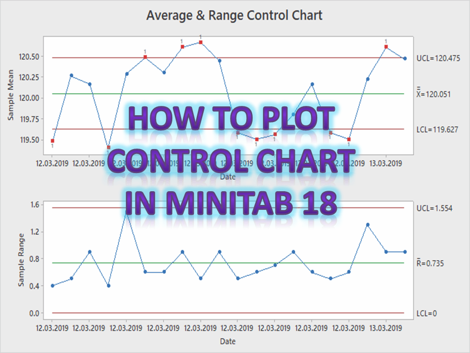
After selecting the data point’s column, subgroup size value, and Label, now you have to enter in “ok”. After doing so Control Chart will appear on the screen.
Minitab Control Chart:
FAQ:
Q1: How to change the
“X” axis value?
A1: Double click on the “X” axis then you can able to see a dialog box where you have to click on the “time” icon (marked in red color box in below figure) then, select the stamp option, and next to select the column which you would like to add in “X” axis.
Shanti Gopal Pradhan is an experienced professional in Quality Management Systems, QA, Operations, Business Excellence, and Process Improvement. He has strong expertise in international standards including IATF 16949, ISO 9001, ISO 14001, ISO 45001, and ISO 17025, along with methodologies such as TQM, TPM, and Six Sigma.
He holds a degree in Mechanical Engineering along with an MBA, combining strong technical acumen with strategic business insight, he is a Certified Internal Auditor, Lead Auditor, and Six Sigma Black Belt, with a proven track record in driving quality transformation and operational excellence.
MTBF and MTTR Template, Format, Calculation| Manufacturing Example:
What is MTBF?
Hi, readers in this article we will be covering both MTBF and MTTR calculation with a manufacturing example. So read carefully, learn the concept, and implement it in your organization. Mean time between failures (MTBF) is the arithmetic average time between failures. It helps to measure the performance of a machine or assets. In manufacturing industries, we are always worried about the breakdown of machine or equipment failure, which can make a large loss and ultimately increase the downtime (Stop time) of the machine. Uptime is a big factor to enhance productivity. The higher the MTBF means the machine runs a long time before failing.
[Figure]
As you can see in the above figure operation has stopped after 8 hours of duration but meanwhile, three failures have occurred. Due to this failure machine was stopped for maintenance. In this case, 8 hours was the available operational time but 6 hours was the total running time. Considering all the above data, the MTBF value is 2 hours. It means the average time between 1st failure & 2nd failure or 2nd failure & 3rd failure is 2 hours. In the manufacturing industry, there are multiple operations and several machines are being used for production. So during the calculation of MTBF, you have to think about multiple factors.
DOWNLOAD– Template of MTBF and MTTR. (mttr, mtbf formula excel)
MTBF Formula:
The total operational time or total run time divided by the total number of failures.
MTBF= (Total Operational Time ÷ Total Number of Failures)
Calculation of MTBF (Mean Time Between Failures):
Let, for example, a product “XYZ” has manufactured in a simple method by using a single machine [see the below figure]. This machine runs three shifts per day with monthly 26 working days. But in last month’s operation, the maintenance person had booked the machine’s total number of failures (Breakdown) was 5. And total break-down time was 3 hours. According to all the above data, Monthly MTBF has been calculated and mentioned below;
[Example-1]
MTBF = Total operational time ÷ Total number of failures
Total operational time (Run time):
= Planned production time – Stop time
(624 hours – Stop time)
= (624- 81), here stop time included the lunch time, dinner time, tea time, breakdown time, tool changeovers time)
=543 hours
Now, the Total Operational Time of last month = 543 hours, Total number of failures of last month =5 times.
MTBF of last month = (543÷5) hours
=108.6 hours
Similarly, we have calculated the MTBF of a complex process having multiple numbers of machines.
[Example-2]
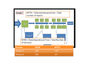
In example 2, all 13 machines run together to produce a product. There is a total of three sub-process i.e. process-1, 2 &3. And process-1 has 1 machine and process-2 &3 have 6 machines each. First of all, we will calculate the MTBF value of each process and then the overall process. Details of data like a machine running time, failure frequency, etc. are given below,
MTBF of Last month:
Total Operation Shift = A, B, C (3 shifts).
Total Number of Machines = 13
Working days of last month = 25 days
Total Number of failures (B/D) =12 times [process-1 =2, process-2 =6, process-3 =4]
Total breakdown time = 10 hours [process-1 =1, process-2 =8, process-3 =1]
Stop time of each machine per day due to Lunch, Dinner, and tea = 3 hours
MTBF of Process-1:
MTBF = Total operational time ÷ Total number of failures
Total operational time (Run time):
= Planned production time – Stop time
(600 hours – Stop time)
= (600- 76)
=524 hours.
Now, Total Operational Time of last month = 524 hours, Total number of failures of last month = 2 times.
MTBF of last month = (524÷2) hours
=262 hours
MTBF of Process-2:
MTBF = Total operational time ÷ Total number of failures
Total operational time (Run time):
= Planned production time – Stop time
(3600 hours – Stop time)
= (3600- 458)
=3142 hours
Now, Total Operational Time of last month = 3142 hours, Total number of failures of last month = 6 times.
MTBF of last month = (3142÷6) hours
=523.666 hours
MTBF of Process-3:
MTBF = Total operational time ÷ Total number of failures
Total operational time (Run time):
= Planned production time – Stop time
(3600 hours – Stop time)
= (3600- 451)
=3149 hours
Now, Total Operational Time of last month = 3149 hours, Total number of failures of last month = 4 times.
It is the average time required to correct and repair a failed component or equipment or device to put it in working order. It reflects how much average time is spent to correct or repair the component.
MTTR Formula:
Total maintenance time or total B/D time divided by the total number of failures.
MTTR = Total maintenance time ÷ Total number of repairs.
MTTR Calculation (Mean time to repair):
Example-3.
It’s a simple manufacturing process consisting of a single machine. In last month 3 times machine was stopped due to breakdown & the total breakdown or repair time was 2 hours. So here we are going to calculate the MTTR, details of the calculation are given below.
[Example-3]
MTTR = Total maintenance time ÷ Total number of repairs.
= (2 ÷ 3)
= 0.67 hours
Example-4:
[Example-4]
In Example-4, the whole process is covered by the two sub-process i.e. process-1 and process-2. In first sub-process has a total of 4 machines and similarly, the second process has a total of 6 machines in operation. All data related to breakdown and frequency of failure are given in below table;
Process
Breakdown or Maintenance time
Frequency of failure or total number of repairs
Process-1
5 hours
3
Process-2
4 hours
6
MTTR of Process-1: 1.67 hours
MTTR of Process-2: 0.67 hours
Overall process MTTR = (1.67 + 0.67) ÷2
=1.17 hours
Process
MTTR in Hours
Process-1
1.67
Process-2
0.67
Overall Process
1.17
MTTR-Table
Why MTBF and MTTR are important for manufacturing industries?
MTTR indicates the efficiency of corrective action of machine failure and similarly
MTBF indicates the average machine run time between failures.
Monitoring both indicators can give the idea to control your maintenance method and indicate the opportunity for improvement in the same field. You can easily identify the training needed for your maintenance personnel after analyzing the values. You can also categorize the production loss w.r.t breakdown time.
What is the requirement of IATF 16949 w.r.t MTBF and MTTR?
As per the standard requirement, an organization shall document the maintenance objectives, for example, the objective of MTTR and MTBF.
How do you calculate MTBF and MTTR?
We have calculated the MTBF and MTTR with a manufacturing example, please read the above example.
What is the MTTR formula?
MTTR = Total maintenance time ÷ Total number of repairs.
How do you calculate MTBF?
MTBF= (Total Operational Time ÷ Total Number of Failures)
How to reduce the MTTR hours and How to increase the MTBF hours?
For improving both the parameters, we have to keep the focus on below things, like
Do the periodic CLIT (Cleaning, Lubrication, Inspection, and tightening).
Do the Kaizen on machines.
provide the training to the maintenance team.
Display the OPL for the machine operators for a better understanding of the machine’s operation.
Visual marking on the machine and introducing the poka-yoke
The above points are not limited to the given list but you can do more best practices to improve the MTTR and MTBF.
Free Templates / Formats of QM: we have published some free templates or formats related to Quality Management with manufacturing / industrial practical examples for better understanding and learning. if you have not yet read these free template articles/posts then, you could visit our “Template/Format” section. Thanks for reading…keep visiting techiequality.com
Shanti Gopal Pradhan is an experienced professional in Quality Management Systems, QA, Operations, Business Excellence, and Process Improvement. He has strong expertise in international standards including IATF 16949, ISO 9001, ISO 14001, ISO 45001, and ISO 17025, along with methodologies such as TQM, TPM, and Six Sigma.
He holds a degree in Mechanical Engineering along with an MBA, combining strong technical acumen with strategic business insight, he is a Certified Internal Auditor, Lead Auditor, and Six Sigma Black Belt, with a proven track record in driving quality transformation and operational excellence.