Control Chart Excel Template |How to Plot Control Chart in Excel | Download Template:
Hi! Reader, today we will guide you on how to plot a control chart in Excel with an example. To take more concentration on Process Improvement, the control chart always takes vital rules to identify the Special causes and common causes in Process Variation. Control Chart Excel Template is available here; just download it by clicking on the
Download the Control Chart Excel Template.
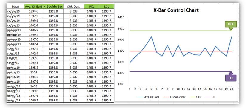
[Figure 1-X- Bar Control Chart Excel Template]
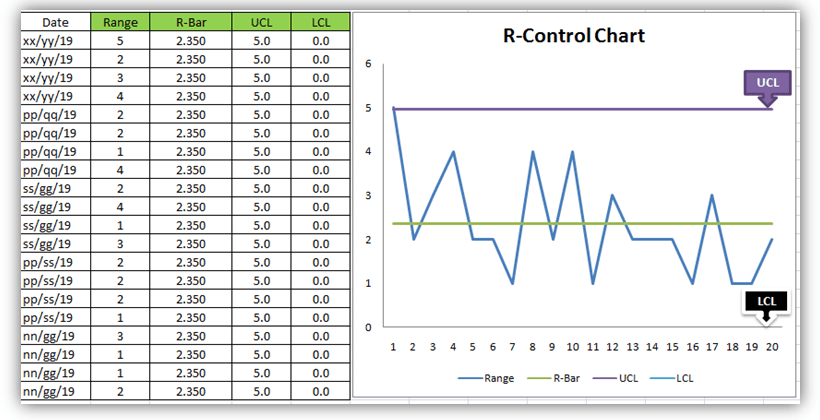
[Figure 2-R-Control Chart Excel Template]
A Control Chart is a graphic representation of a characteristic of a process, showing plotted values of some statistic gathered from that characteristic, a centerline, and one or two control limits. It has two basic uses as an adjustment to determine if a process has been operating in statistical control and to aid in maintaining statistical control.
Control Chart Approach for Continual Process Improvement:
- Data Collection.
- Control.
- Analysis and Improvement.
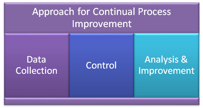
- Data Collection:-
- To Collect Data and Plot the Control Chart.
- Control:-
- Calculate control limits from process data.
- Identify Special Causes of Variation and Act upon them.
- Analysis & Improvement:-
- Quantify Common Cause Variation, and take action to reduce it.
You will also like to read the CAPA Process
7QC Tools for Problem Solving | What are 7 QC Tools
How to Plot Pareto Chart in Excel ( with example)
How to Create Control Chart Excel Template| Step-by-Step Guides (X-Bar & Range Chart) with Example:
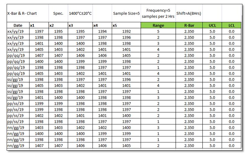
Step-1: Collect The Data day-wise/shift-wise.
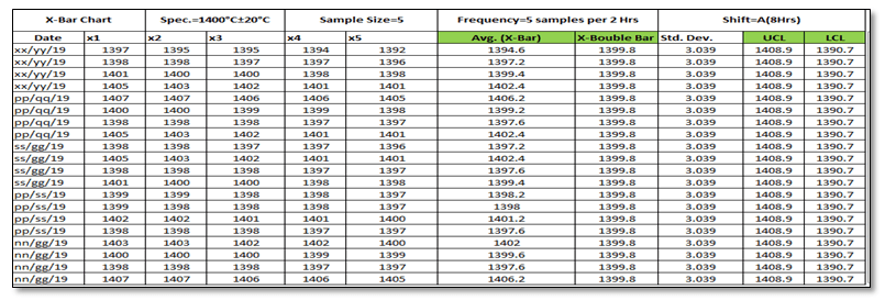
As you can see in the above figure, we have collected data with a sample size of 5 for A-Shift with frequency (5 samples per 2 hours). So we have only one shift data for 5 days. Total 100 number observations. You are supposed to collect the data as per the Control Plan or Quality Assurance Plan.
Step-2: Select the Data types and applicable Control Chart.
So we have variable type data and the
Step-3: According to data type and Sample size, presently we are going to plot the X-Bar & R-Chart. So individually we will plot both charts (X-Bar Chart & Range Chart). First, we will plot the X-bar chart and then the R-chart.
3.1 X-Bar Chart:

Before we start, just go through the green highlighted terms in the above figure as [1] Average
[2] X-Double Bar means an average of average. [3] Standard Deviation. [4] UCL. [5] LCL.
Calculation:
[1] Average:
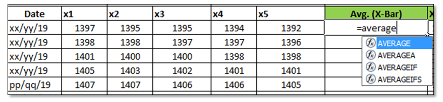
Make sure that your attention is now on the right side corner of the above figure. To calculate the average value of individual subgroup size. You have to type as (=average)and then double click on the average function and next select the sample value from x1 to x5.
[2] X-Double Bar: After calculating the Average value of all Subgroups (Individual Date wise), now we have to calculate the average of Average (Average of X-Bar).
[3] Standard Deviation: Standard Deviation of Average (X-Bar),
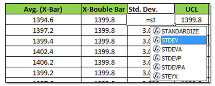
Type as (=Stdev) and select all X-Bar Data to Calculate the Std. Dev. of Average.
[4] UCL:
UCL=X Double Bar +3*Sigma
UCL= X Double Bar +3*Standard Deviation
For the calculation of the UCL in Excel use the above formula.
[5]LCL:
LCL=X Double Bar -3*Sigma
LCL= X Double Bar -3*Standard Deviation
Use the above Formula in Excel.
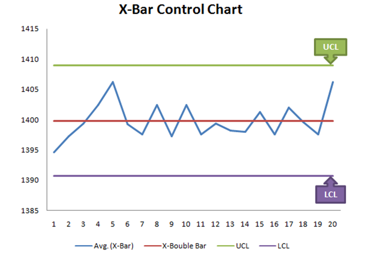
3.11 Plot X-Bar Chart: This is the last step to plot the X-Bar Chart by using Line Graph in Excel, follow the below steps:
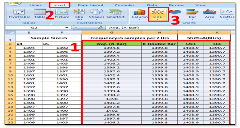
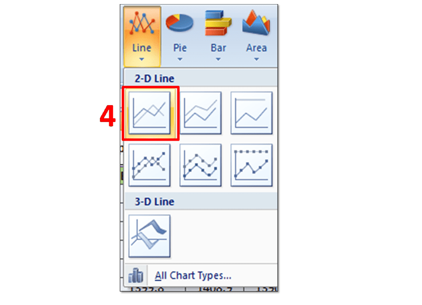
Simply Follow Sl. No.1 to 4.
In Sl. No.1, Select X-Bar, X-Double Bar, UCL, LCL, and then select Insert Option and next to Line Chart. After selecting the Line Graph/Chart, The X-Bar Control Chart Excel Template will be ready as below.
3.2 Range Chart:
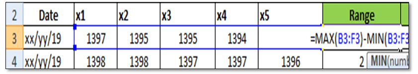
To Plot the R-Control Chart, we have to calculate the [1] Range. [2] R-Bar (Average of Range). [3]UCL. [4]LCL.
[1] Range: R=Max. Value – Min. Value of Subgroup.
[2] R- Bar (Average of Range): Put the Excel formula of average.
[3] UCL:
UCL= D4 x R-Bar
UCL= 2.114 x R-Bar Value of individual Subgroup. (Note for Subgroup Size 5, D4=2.114).
Use this formula in Excel to calculate the UCL.
[4] LCL:
LCL=D3 x R-Bar
LCL=0 (Note Foe subgroup size 5, D3=0)
Simply put the “0” in the Excel sheet.
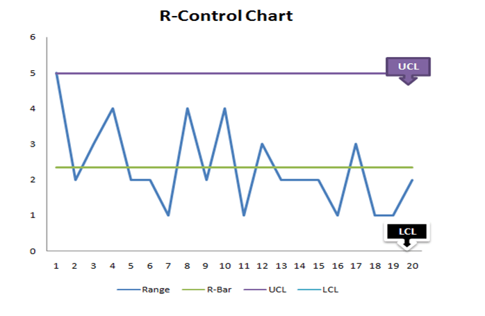
3.22 Plot R-Chart: Just follow steps 1 to 3, and select the line chart.
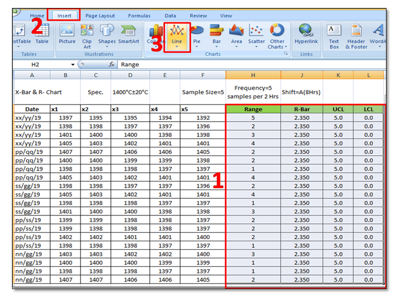
In step-1, you have to select the “Range, R-Bar, UCL, and LCL” simultaneously and then select the Line Chart, after selecting the line chart R-Control Chart Excel Template will be ready as below
FAQ:
Q1: What are control chart rules?
A1: Read the full article “What is SPC”.
Q2: How to add upper and lower control limits in Excel?
A2: Carefully read the aforesaid Articles.
Q3: How to create a control chart in Excel 2013?
A3: Step by Step guide is described above with Statistical process control chart examples. Please go through it.
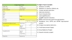
Q4: How to create a Six Sigma control chart in Excel?
A4: Control charts are classified into two types [1] Variable type and [2] Attribute Type. Both two types are further classified into several as
[1]Variable types
- X and MR Chart
- X-Bar and Range
- X-Bar and S
[2] Attribute Chart
- np-chart
- p-chart
- u-chart
- c-chart
In the above articles, we have described only how to create an X-bar and range type Control Chart in Excel with a process control chart example. As you can see all these above types of control charts are used in Six Sigma projects but the applicable chart depends on Data type and Subgroup size (Sample size).
Q5: How to calculate upper and lower control limits (UCL & LCL) in Excel?
A5: For X-Bar Chart-UCL:
UCL=X Double Bar +3*Sigma
UCL= X Double Bar +3*Standard Deviation
For the calculation of the UCL in Excel, use the above formula.
LCL:
LCL=X Double Bar -3*Sigma
LCL= X Double Bar -3*Standard Deviation
Use the above Formula in Excel.
For R-Chart:
UCL:
UCL= D4 x R-Bar
UCL= 2.114 x R-Bar Value of individual Subgroup. (Note for Subgroup Size 5, D4=2.114).
Use this formula in Excel to calculate the UCL.
LCL:
LCL=D3 x R-Bar
LCL=0 (Note Foe subgroup size 5, D3=0)
Simply put the “0” in the Excel sheet.
Q6: What are the types of control charts?
A6: [1] Variable types
- X and MR Chart
- X-Bar and Range
- X-Bar and S
[2] Attribute Chart
- np-chart
- p-chart
- u-chart
- c-chart
Useful Articles:
More on TECHIEQUALITY


Thank you for reading…….keep visiting Techiequality.Com
I hope the above article is useful to you…
Popular Post:

Shanti Gopal Pradhan is an experienced professional in Quality Management Systems, QA, Operations, Business Excellence, and Process Improvement. He has strong expertise in international standards including IATF 16949, ISO 9001, ISO 14001, ISO 45001, and ISO 17025, along with methodologies such as TQM, TPM, and Six Sigma.
He holds a degree in Mechanical Engineering along with an MBA, combining strong technical acumen with strategic business insight, he is a Certified Internal Auditor, Lead Auditor, and Six Sigma Black Belt, with a proven track record in driving quality transformation and operational excellence.