P Chart Excel Template | Formula |Example | Control Chart | Calculation

P Chart Excel Template

P Chart Excel Template | Formula | Example | Control Chart | Calculation

Hi Readers! Here, we are going to discuss on attribute type control chart, especially on the P chart. Also, you can learn the formula, and calculation part with industrial or manufacturing examples. You can download the P chart excel template from below given link.

Sample P chart excel template with industrial example-Download Here

Attribute type Control chart (P Chart):

The P chart, attribute type control chart, or proportion nonconforming chart is generally used to identify the common or special causes present in the process and also used for monitoring and detecting process variation over time. It helps to determine whether the process is in a state of statistical stable or not. Overall, it indicates that special causes are present in the process or not, whether the process is under control or not, and process variability.
How to select proportion nonconforming (P chart):

Step-1: Data Types?

Ans.:- Discrete type data (Attribute type data)

Step-2: Is the interest in nonconforming units or one defect per unit?

Ans.:- yes, one defect per unit

Step-3.:- Is the sample size constant?

Ans.:- Yes or No, then use P chart.

Note; for both the cases, if the sample size is constant or if not, in this scenario you can select p chart.

Data Type:——Discrete type data (Attribute type data)
Is the interest in nonconforming units or one defect per unit?—-Yes
Is the sample size constant?Yes or No
Select Chart type:P Chart

P Chart Formula:

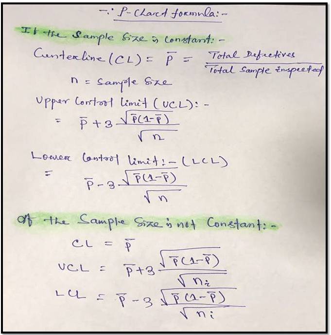
For plotting the P chart in excel we have to calculate the three important things i.e. [1] Center line, [2] Upper control limit, & [3] lower control limit.

P Chart Excel Template
[P Chart Formula]

P chart example & Calculation for constant sample size:

In a manufacturing unit producing the auto part products, a process quality engineer would like to monitor the process control, so he started to collect the data for 30 days and daily inspected 250 products & recorded the defectives or nonconforming parts (Defects-blow hole, shrinkage, pinhole, etc.). 30 days data is given in below table.

DateConstant sample size (n)Defective/
Nonconforming
12501
22502
32502
42501
52502
62501
72500
82501
92504
102502
112503
122501
132500
142503
1525010
162501
172504
182503
192502
202501
212503
222502
232501
242503
252502
262502
272501
282502
292503
302501

With the help of the above data, we are going to calculate and plot the P chart. As we know that we have to calculate the 3 important things, Center line, upper control limit & lower control limit.

Center Line (CL)-P bar: – Total Defectives/ Total sample Inspected

= 64/ (30*250)

= 0.0085

=0.009

Upper Control limit (UCL):-

= P bar+3*square root of (p bar*(1-p bar)/sample size)

= 0.009+3* square root of (0.009*(1-0.009)/250)

=0.009+3*0.005972

=0.026

Lower Control Limit (LCL):-

= P bar-3*square root of (p bar*(1-p bar)/sample size)

= 0.009-3* square root of (0.009*(1-0.009)/250)

=0.009-3*0.005972

= -0.0089

= -0.009

0 (Note: The LCL value is negative, so the final value of LCL is zero)

Now, you have to calculate the proportion defective or nonconforming

Proportion defective:

Here, I’m calculating the proportion defective of day-1, so similarly you can calculate for next day onwards

= Day-2 Defects/Sample size

= 1/250 = 0.004

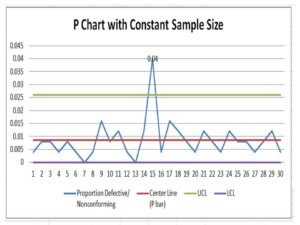
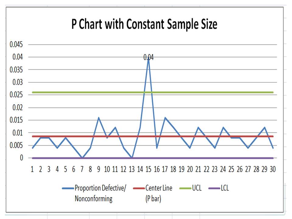
Now, Based on the above data i.e. proportion defects, center line, upper control limit, and lower control limit, we have plotted the P chart in Excel. If you would like to download the p chart excel template with the same calculation then, download it from the above given link and similarly you can download the other template or format by Click Here

P Chart Excel Template
Interpretation of P Chart:

In the above p chart, we have seen that one proportion defect value is beyond the upper control limit. It means on day-15 special cause is present so, we have to take the action on it to control the process.

Free Templates / Formats of QM: we have published some free templates or formats related to Quality Management with manufacturing / industrial practical examples for better understanding and learning. if you have not yet read these free template articles/posts then, you could visit our “Template/Format” section. Thanks for reading…keep visiting techiequality.com

More on TECHIEQUALITY

Popular Post

C Chart Excel Template | Formula | Example | Calculation

C Chart Excel Template

C Chart Excel Template| Formula |Example |Calculation:

Hi Readers! Today, we will be discussing here on attribute type SPC chart i.e. C chart. Its formula, calculation, and industrial example. The C chart is also called the number of nonconformities chart. Where the sample size is constant. Read the below description to learn about its selection and application in industries. If you are interested in downloading the sample C Chart Excel Template then, click on the given below link.

Sample C Chart Excel Template with industrial example-Download.

Number of nonconformities chart (C Chart):

The C chart, attribute type SPC control chart, or the number of nonconformities chart is generally used to identify the common or special causes present in the process and is also used for monitoring and detecting process variation over time. It helps to determine whether the process is in a state of statistical stable or not. Overall, it indicates that special causes are present in the process or not, whether the process is under control or not, and process variability. This C chart is selected when there is a constant sample size and multiple defects per unit are present.

Selection of Attribute type SPC Control chart (C Chart):

Step-1: Data Types?

Condition: – Discrete type data (Attribute type data)

Step-2: Is the interest in nonconformities or multiple defects per unit?

Condition: – yes, multiple defects per unit

Step-3.:- Is the sample size constant?

Condition: – Yes, then use the C chart.

DescriptionCondition
Data Type:Discrete type data (Attribute type data)
Is the interest in nonconformities or multiple defects per unit?Yes, Multiple defects per unit present
Is the sample size constant?Yes
Chart type:C Chart

C Chart Formula:

The three important things need to be calculated before plotting the C chart i.e. [1] Centerline, [2] Upper control limit, & [3] lower control limit.

Centerline (CL) or C bar = Total number of nonconformities or defects / Number of samples

Upper control limit (UCL) = C-bar + 3 x Square root of C-bar

Lower control limit (LCL) = C-bar – 3 x Square root of C-bar

 The formula of C chart
CL or C- bar =Total number of nonconformities or defects / Number of samples
UCL =C-bar + 3 x Square root of C-bar
LCL =C-bar – 3 x Square root of C-bar

How to plot a c chart in excel?

Here, I’m going to share my own industrial experience regarding the application and usage of a c chart in the manufacturing industry by providing a sample example for your quick learning and implementation in your organization. I have considered 50 sample sizes, and three different defects and collected the data for 30 days. Details of data are given below table.   

DateConstant sample size (n)Defect-1Defect-2Defect-3Total Defects
15011 2
2501124
3502215
45011 2
5501124
65011 2
7501113
8502226
9502237
10501124
11501135
12501113
135055717
145011 2
15501113
16502215
175011 2
18501113
19501135
205011 2
215022 4
225011 2
23502226
24501135
25501113
265022 4
27501113
285011 2
29501113
30501113

All the above three defects are attribute type defects. Before plotting the c chart in excel we have to calculate the three important things first, one is CL, UCL & LCL.

Calculation:

Centerline (CL) or C-bar:

Formula = Total number of nonconformities or defects / Number of samples

CL = 121 / 30 =4.033

UCL (Upper control limit):

Formula = C-bar + 3 x Square root of C-bar

UCL = 4.033 + 3* Square root of 4.033

UCL = 4.033+3*2.008

UCL = 10.0577

UCL = 10.058

LCL (Lower control limit):

LCL = C-bar – 3 x Square root of C-bar

LCL = 4.033 – 3* Square root of 4.033

LCL = 4.033-3*2.008

LCL = 4.033-6.024

LCL = -1.991 (the value is negative so LCL is Zero)

LCL = 0.00

 Calculation value
CL =4.033
UCL =10.058
LCL =0
Follow the below step to plot the c chart in excel:

Step-1: open the excel sheet.

Step-2: Do the data entry on the Excel sheet.

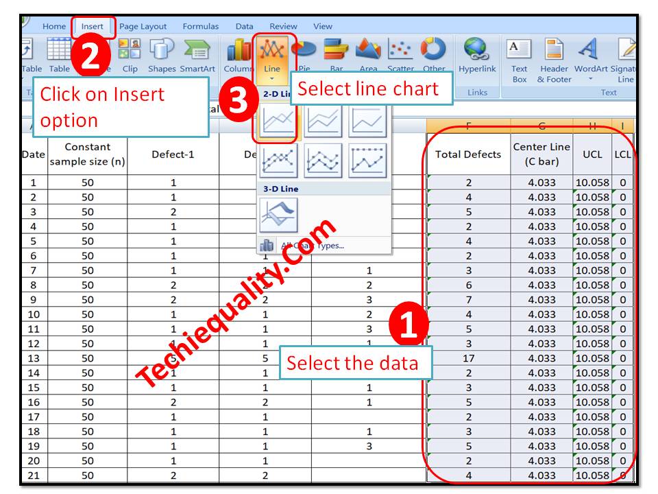
Step-3: Select the data and then go to the insert option in the main menu and next to select line chart. The detail is mentioned in the below image.

C Chart Excel Template
C Chart:

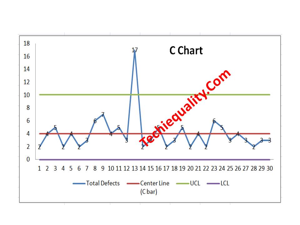
With the help of the above data, we have plotted the c chart, which is given below. if you would like to download the C Chart Excel Template then, click here.

C Chart Excel Template
Interpretation of the above C Chart:

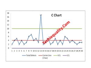
In the above C chart, we have seen that one defect value is beyond the upper control limit. It means on day-13 special cause was present in the process, so we have to take the action on it to control the process.

Free Templates / Formats of QM: we have published some free templates or formats related to Quality Management with manufacturing / industrial practical examples for better understanding and learning. if you have not yet read these free template articles/posts then, you could visit our “Template/Format” section. Thanks for reading…keep visiting techiequality.com

Useful Post:

What is Preventive Maintenance? | Predictive Maintenance |Types & Example

Plan Do Check Act Cycle | PDCA Cycle Manufacturing Example | Implementation

Attribute MSA |How to do Attribute type MSA Study| Example |Acceptance Criteria

Gage R and R |Attribute type MSA |How to do MSA Study | Acceptance Criteria

More on TECHIEQUALITY

4M Change Management | How to implement in Manufacturing unit | Template | Format

4M Change Management

4M Change Management| How to implement in Manufacturing unit |Template | Format

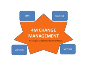
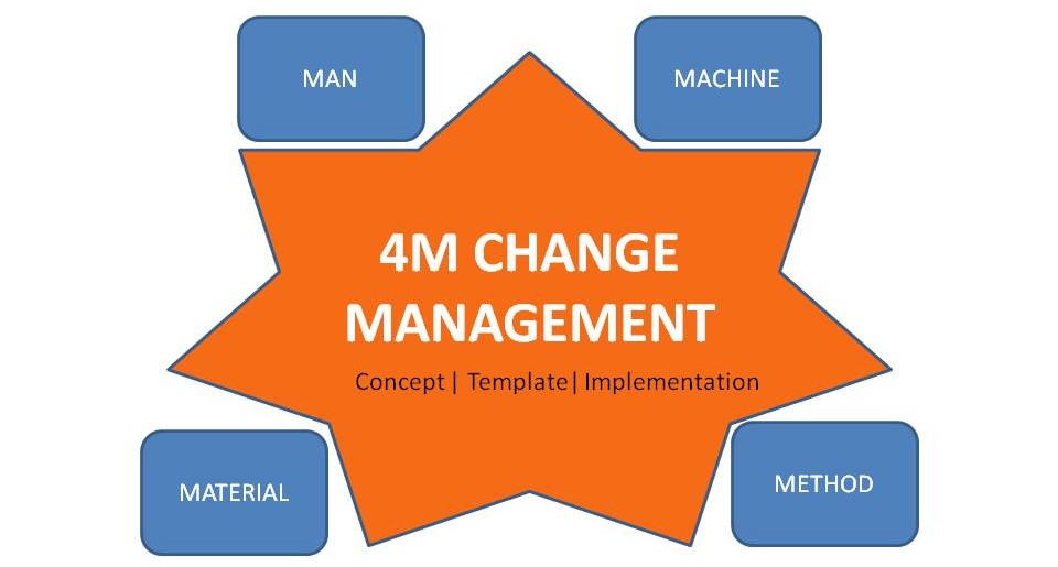
Hi Readers! Today here, we are going to discuss 4M Change management related to manufacturing industries with an illustration. You can learn many more things from this article like 4M change concepts, planned and unplanned changes, implementation of concepts in your organization, etc. The concept of 4M change management is generally used to record 4M (man, machine, method & material) related to planned and unplanned changes. This can apply to all internal process changes.

Download the 4M checklist for gap analysis.-4M Checklist-DOWNLOAD

4M Change Management

As we already discussed 4M changes i.e. Man, Machine, Method & Material related planned and unplanned changes. so here, first of all, we have to understand, what planned and unplanned changes are. The plan changes that occur with the advanced information to the pertinent personnel. Similarly, the un-plan change that occurs without prior information to the pertinent person. If once the planned and unplanned changes occurred then a defined action which is mentioned in SOP/Procedure is required to control the occurrence of nonconformity at the shop floor change area.

Illustration / Example (How to implement 4M change management in manufacturing Unit?):

Example of plan change:

Let’s say an organization has planned for preventive maintenance of machine-1 in shift –A, dated xx/1/20xx, and executed the same as per plan. If so then how to record the same 4M change and control the process after PM.

Before implementing 4M change management, personally, I would recommend that try to prepare the procedure /SOP as per your organization’s nature of production, like the 4M procedure, change tracking record, list of trained operators, list of machines, material list, etc.

According to the above example scenario, we are going to record the 4M change in the below template (this template is only for reference)
DateMachineShiftType of changeDetails of changeAction taken
xx/1/20xxmachine-1APlanned / machinePreventive maintenanceSet up approval checking

 In this way, you can maintain the change record. For your better understanding and more clarification, we have given below another example related to the unplanned 4M change.

Example of un-plan change:

 For example, an operator on leave without prior information to the pertinent supervisor and you as a supervisor planned for running the machine-1 with the help of other operators. In that scenario, how to record the 4M change, and what action is to be taken?

Similarly, we are going to record the un-plan change as per the above 4M change template or format.

DateMachineShiftType of changeDetails of changeAction taken
xx/1/20xxmachine-1AUn-planned /ManThe operator is on leave without intimationA similar skilled operator will run the machine/machine setup approval to be done

The 4M change record can be helpful for analysis in the future if there will be any issues with the product. And the action you have taken at the time of the 4M change can control the process as proactively.

I hope the above example is meaningful for your better learning and understanding related to 4m change management implementation in your organization.

Example of Abnormality ( Abnormal situation handling):

It is very important to understand all three situations/changes i.e. [1] plan change, [2] un-plan change, [3] abnormality. now here we are going to discuss the 4M change management of abnormal situation handling (abnormality). Suppose in a production line, a machine-1 on a sudden breakdown, for this situation we are going to record the 4M change, and the same is given below.

DateMachineShiftType of changeDetails of changeAction taken
dd/mm/yymachine-1B-shiftAbnormality /MachineMachine-1 on sudden breakdown1) Run a backup machine, if available.
2) Do the setup approval & Retroactive inspection
3) Containment action.

Free Templates / Formats of QM: we have published some free templates or formats related to Quality Management with manufacturing / industrial practical examples for better understanding and learning. if you have not yet read these free template articles/posts then, you could visit our “Template/Format” section. Thanks for reading…keep visiting techiequality.com

Useful Post:

C Chart Excel Template | Formula | Example | Calculation

P Chart Excel Template | Formula |Example |Control Chart | Calculation

Variation Calculation in Excel | Types of Variation |Manufacturing Example

Equipment Ranking Process | A B C Ranking of Machine with Manufacturing Example

More on TECHIEQUALITY

SIPOC Template | SIPOC Diagram Example of Manufacturing & Service Industry

SIPOC Template

SIPOC Template | SIPOC Diagram Example of Manufacturing & Service Industry

Hi Readers! Today here, we will be discussing on SIPOC template and examples of sipoc diagrams of manufacturing and service industries. As you know that SIPOC is one of the most useful diagrams which is generally used for a better understanding of the process. In both the manufacturing and service industries are commonly used the two types of process mapping diagrams are. I.e. [1] PFD- Process flow diagram and another [2] SIPOC diagram. If you would like to download the free SIPOC excel template then, click on the given below download link.  

Download the SIPOC template in excel format-SIPOC Excel format-DOWNLOAD Link

What is SIPOC Diagram?

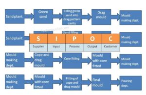
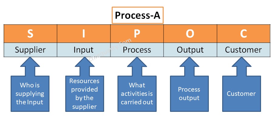
The SIPOC diagram consists of 5 elements i.e. [1] Suppliers, [2] Inputs, [3] Processes, [4] Outputs, [5] Customers. The diagram is generally used for process mapping. It helps to understand the overview of the process in detail.

5 Steps to create a SIPOC Diagram:

Step-1:

Create a CFT team including the process owner of a particular process, which you are trying to draw.

Step-2:

Define the process, for example, let’s consider a process namely called Process-A and you are trying to draw an SIPOC diagram, so first of all you are supposed to list out the details activities of process-A in sequence with the help of the CFT team.

Step-3:

After listing out the details process sequence, find out the internal and external suppliers. Details are mentioned below example.

Step-4:

List out and identify the inputs, process, process output and then customers

Step-5:

 Draw the Diagram by entering the above points in the appropriate places.

SIPOC Template

[SIPOC Template / Format]

SIPOC Diagram vs PFD – process flow diagram:

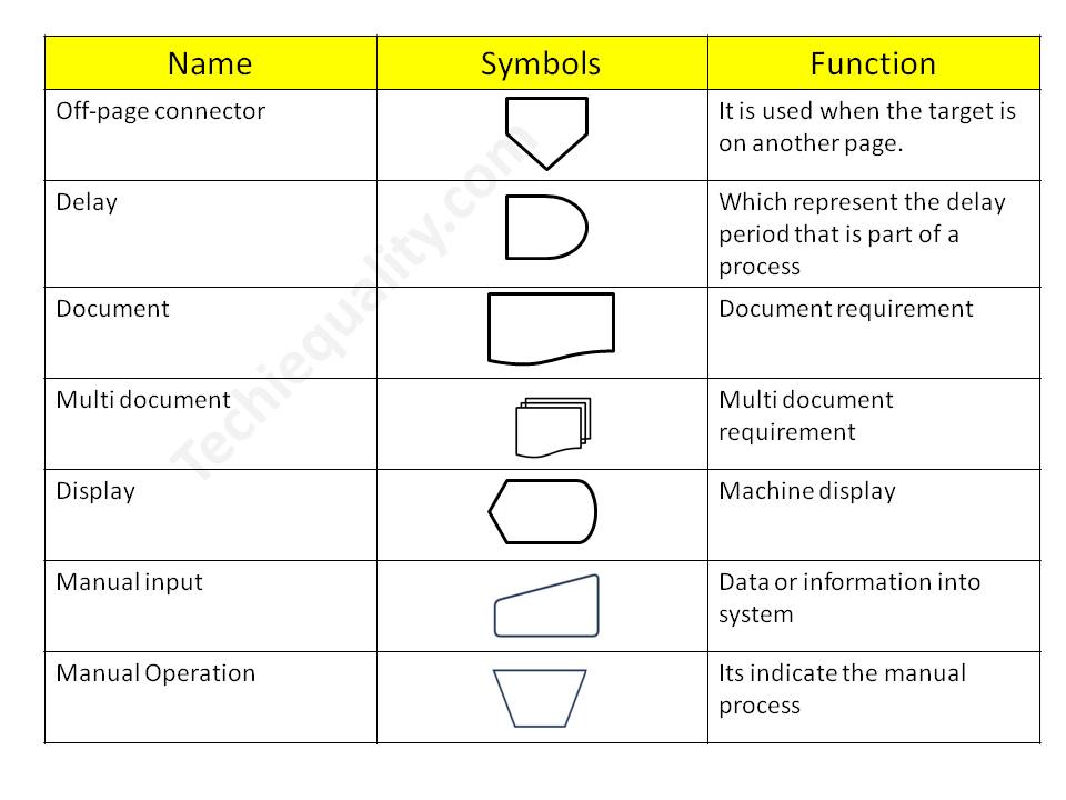
Both the SIPOC diagram and process flow diagram are used to represent the process mapping but the difference between the two is the elements that are used to represent the process details. In SIPOC, we use the 4 elements like supplier, input, process, output, and customer but in PFD, we use flow chart symbols, like the terminator, process, flow line (arrow connector), decision, document, connector, data, preparation, off-page connector, etc.

SIPOC Diagram Example of Manufacturing & Service Industry:

Manufacturing Industry Example:

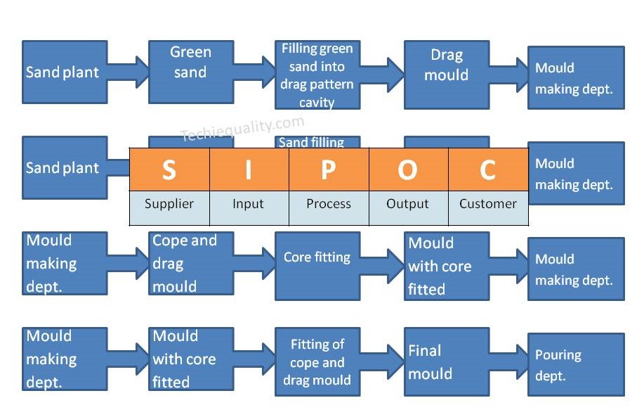
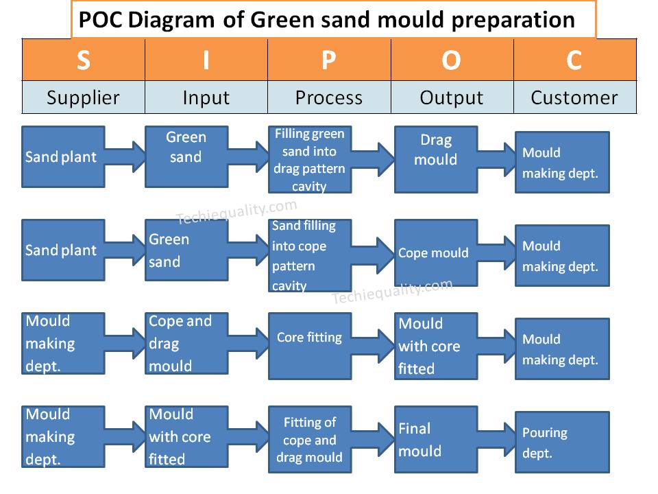
Suppose a company manufactures automobile parts through foundry technology and they have planned to prepare a SIPOC diagram of one of the processes called green sand mould preparation.

SupplierInputProcessOutputCustomer
Sand plantGreen sandFilling green sand into drag pattern cavityDrag mouldMould making dept.
Sand plantGreen sandFilling green sand into cope pattern cavityCope mouldMould making dept.
Mould making dept.Cope and drag mouldCore fittingMould with core fittedMould making dept.
Mould making deptMould with core fittedFitting of cope and drag mouldFinal mouldPouring dept.
SIPOC Template
Service Industry Example:

Let’s consider one of the service sectors of finance as an example bank, and we are going to draw a SIPOC diagram of an offline saving bank account opening process, which is given below;

SupplierInputProcessOutputCustomer
…..Application filled-up formOffline checking and verification of documents deposited by the customerVerified documentDocument verification document
Document verification dept.Verified documentAccount creationNew saving bank account numberAccount creation dept
Account creation deptNew saving accountPassbook issuingNew passbookMr. XYZ
FAQ:

What does sipoc stand for in Six Sigma?

Ans.: The SIPOC stands for Supplier, Input, Process, Output and Customer.

What is a SIPOC template?

The SIPOC template is a diagram which consists of suppliers, inputs, processes, outputs and customers. With the help of the SIPOC diagram, you can prepare the details process flow from start to end.

Free Templates / Formats of QM: we have published some free templates or formats related to Quality Management with manufacturing / industrial practical examples for better understanding and learning. if you have not yet read these free template articles/posts then, you could visit our “Template/Format” section. Thanks for reading…keep visiting techiequality.com

Useful Post:

How to Choose the Best Forecasting Method| Marketing & Sales Example

Variation Calculation in Excel | Types of Variation |Manufacturing Example

Plan Do Check Act Cycle | PDCA Cycle Manufacturing Example | Implementation

Turtle Diagram Example | QMS Standard Requirement |Free Template |Format.

More on TECHIEQUALITY

Equipment Ranking Process | A B C Ranking of Machine with Manufacturing Example

Equipment Ranking Process

Equipment Ranking Process | A B C Ranking of Machine with Manufacturing Example:

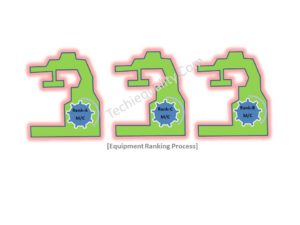
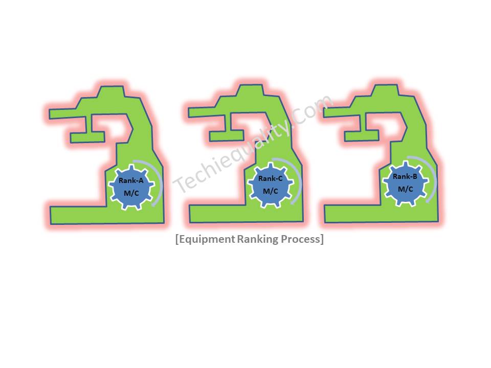
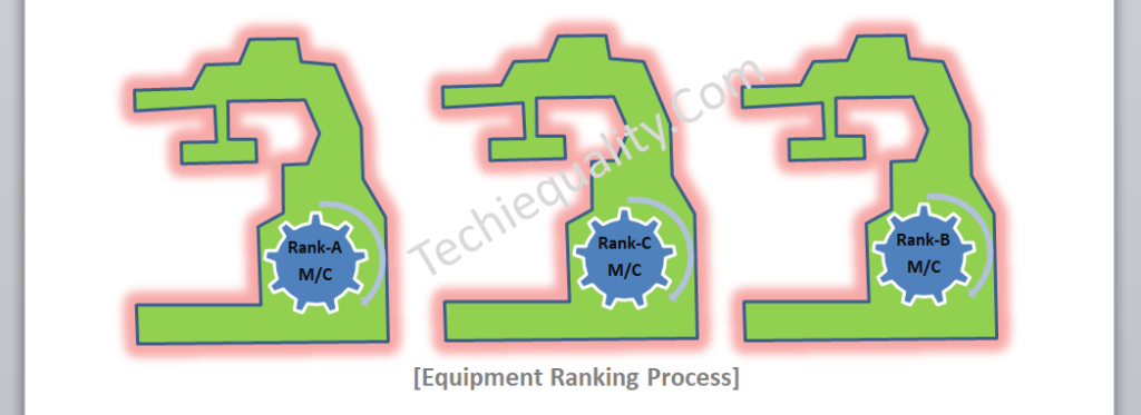
Hi readers! Today we are going to discuss on equipment ranking process, it is an important part of the maintenance process, where machines/equipment/ parts will be ranked and based on the rank category, and you can easily set up the maintenance principle. The organization will get benefits in terms of productivity, quality, cost, safety, etc., and also it will help you to select the type of maintenance applicable / applied on which machine.

Equipment Ranking Process:

Equipment Ranking Process

If first time, you are going to implement it in your organization then you have to formalize many more things like SOP, Check-sheet, list of equipment/ machine, machine /equipment ranking criteria, data, etc. so here, we will help you for easy implementation of this process.

Step by step process has been defined below to implement the machine /equipment ranking process in your manufacturing organization;

Step-1: Prepare the SOP, List of equipment, and equipment/machine ranking criteria procedure.

In the ranking criteria, you can consider the PQCDS means Production, Quality, Cost, delivery, and safety as weightage for factors in categorization, but some industry also considers other factors like Maintenance / Maintainability, Operability, etc.

All the above factors are not equally important and they vary from industry to industry based on the application, material used, quality, safety, etc. For example, equipment is being used for chemical handling, safety factors get a high weightage for rating calculation. And similarly, imported machines may come under high weightage on maintainability if spare parts are mostly imported procurement may take more time and the cost of repair could be high.

Step-2: Form a CF-Team, including Production, quality, maintenance, and safety personnel for best weightage consideration.

For example, let’s say we are having total of 16 machines, and according to their criticality w.r.t PQCDSM and consultation with CF-Team, finally, we have broadly done the weightage of factors of individual machines or similar types of machines.

Machine-1
P-Production100
Q-Quality100
C-Cost50
D-Delivery50
S-Safety20
M-Maintainability20
Total =340
[M/C-1 Data Table-1]

Machine-2

P-Production100
Q-Quality90
C-Cost50
D-Delivery40
S-Safety40
M-Maintainability40
Total =360
[M/C-2 Data Table-2]
Machine-16
Production-P100
Quality-Q80
Cost-C50
Delivery-D40
Safety-S40
Maintainability-M40
Total =350
[M/C-16 Data Table-3]

Similarly, you can do the weightage of factors of all machines or you can prepare the common criteria sheet for similar types of Machines.

Step-3: Prepare the final ranking criteria sheet.

For example, we have prepared the below-ranking criteria sheet for reference only, you can prepare according to your organization’s decision and machine’s factors, operations, etc. but here we have made the generic criteria rules is given below.

Let’s say “Quality” factors have 100 marks and we have divided them into four degrees of factors.

Mark=100806040
Always being required to work to a very fine tolerance or Equipment failure mode has a major effect on quality, the product produced out of Specification.Produce quality variations, some of the products may get rejected but the operator’s intervention requires less time to correct it.The Product can be reworked and used, meets the specification and drawing, machine is sufficiently accurate for required tolerance.No quality problems, no effect on quality, and no product defects.
[Ranking Criteria Matrix]
 Accordingly, you can prepare the ranking criteria matrix for Production, cost, safety, delivery, and maintainability, etc.

Let’s consider the machine-1, factors given in above i.e.

P-Production100
Q-Quality100
C-Cost50
D-Delivery50
S-Safety20
M-Maintainability20
Total =340

The total mark of the entire above factor (PQCDSM) is 340.  Based on the organization’s decision and degree of factors mark, an organization can decide the range for the category of machine, e.g.

Up to 130 marks ——-C Rank / Category

131 to 190 marks ——-B Rank / Category

191 to 340 marks ——- A Rank / Category

As you know that we have considered 16 machines, so our CF-team members have collected and gathered the machine history records, data and with the help of the ranking criteria matrix, they have evaluated the entire machine, and the same is mentioned below the table.
MachineRank / Category
M/C-1A
M/C-2B
Machine-3C
M/C-4C
M/C-5A
Machine-6B
M/C-7A
Machine-8B
M/C-9B
Machine-10B
M/C-11A
Machine-12B
M/C-13B
Machine-14A
M/C-15C
Machine-16C
[A B C Ranking Table]

According to the machine’s rank, you have to prepare the maintenance plan, e.g. our maintenance engineer has decided that M/C-1 will be covered under preventive and predictive maintenance twice a month and similarly M/C-8 will be covered under preventive maintenance twice a month. And M/C-16 may be covered under preventive maintenance once a month or only BM. So, in this way, you can prioritize the machine maintenance period w.r.t m/c or equipment category or ranking.

Free Templates / Formats of QM: we have published some free templates or formats related to Quality Management with manufacturing / industrial practical examples for better understanding and learning. if you have not yet read these free template articles/posts then, you could visit our “Template/Format” section. Thanks for reading…keep visiting techiequality.com

Useful Post:

What is Preventive Maintenance? | Predictive Maintenance |Types & Example

Plan Do Check Act Cycle | PDCA Cycle Manufacturing Example | Implementation

Attribute MSA |How to do Attribute type MSA Study| Example |Acceptance Criteria

Gage R and R |Attribute type MSA |How to do MSA Study | Acceptance Criteria

More on TECHIEQUALITY

Variation Calculation in Excel | Types of Variation | Manufacturing Example

Variation Calculation in Excel

Variation Calculation by Excel | Types of Variation | Manufacturing Example:

Hi readers! Today we are going to calculate the different types of Variation with the help of Excel. Here we will learn the complete calculation of variation with industrial examples. All the calculations related to variation are done here with the help of the excel-2007 version, the positioning and terminology may be varied w.r.t other versions of Excel. But anyway variation calculation in excel-2007 version will give you a complete idea so you can easily apply the concept in any version of Excel as well.

This topic will help you to enhance your knowledge so that you can easily solve the problem related to variation calculation and the important things that, if you are working in the manufacturing industry and if you would like to know the data variation of process or product characteristics then by using of excel sheet easily you can calculate the variation of the data set.

Variation Calculation in Excel:

First of all, we are supposed to know that what is Variation. I mean to say that Variation is nothing but a way to show how the data is spread out, which means how the data are spread over a wide area.

Types of Variation:

There are so many ways to measures the variation but some common measures of variation used in statistics are;

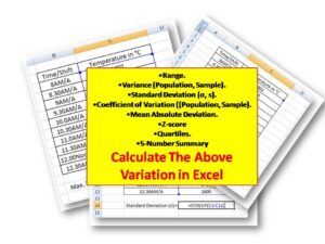
  1. Range.
  2. Variance (Population, Sample).
  3. Standard Deviation (σ, s).
  4. Coefficient of Variation ((Population, Sample).
  5. Mean Absolute Deviation.
  6. Z-score
  7. Quartiles.
  8. 5-Number Summary

We will be calculating all the above measures of variation with the manufacturing example so that you can easily understand and implement the concept in your manufacturing process to know the variation of the data set.

Manufacturing Example to Calculate the Different Measures of Variation:

Let’s a company m/s PQR manufacturing the product “X”. A Quality Engineer Mr. P monitoring the process parameter as per the QA plan, but one day during the shop floor visit, the QA head observed that the process parameter of temperature reading was on the higher side, so he immediately called to process QA engineer and asked to calculate the different measurement of the variation of last period data set. Accordingly, the Process QA engineer had started the calculation, details are given below;

Data: Specification of Temperature: 1400±10°C

Time/ShiftTemperature in °C
8AM/A1402
8.30AM/A1405
9AM/A1401
9.30AM/A1400
10.0AM/A1405
10.30AM/A1403
11.0AM/A1406
11.30AM/A1401
12.00Noon/A1404
12.30AM/A1400
[Temperature reading table]

Here, we are going to calculate the first Range of all the above data sets.

Range = (Maximum Value – Minimum Value)

How to Calculate Range in Excel?

Step-1: Open the Excel Sheet

Step-2: Type the Data.

Variation Calculation in Excel

Step-3: Use the “MAX” function to find out the maximum value, see the below picture to learn more

Variation Calculation in Excel

The Maximum value, we found from the above data set is 1406°C and similarly calculated the minimum value as per the below process as.

Variation Calculation in Excel

Found, the minimum value is 1400°C.

Range = (Maximum Value – Minimum Value)

=1406-1400=6°C

VARIANCE:

variance calculation

Excel-2007 function of Variance for population = VARP(data range)

The Variance of the above population data is 4.41, enter the same data in your excel sheet and calculate & check whether you are getting the same value or not.

Standard Deviation (σ):

standard deviation

Standard Deviation (σ)excel-2007 function=STDEVP(Data range)

(σ) The standard Deviation of the above data set is 2.1, check whether you found the same value in your excel sheet or not using the above data set.

Free Templates / Formats of QM: we have published some free templates or formats related to Quality Management with manufacturing / industrial practical examples for better understanding and learning. if you have not yet read these free template articles/posts then, you could visit our “Template/Format” section. Thanks for reading…keep visiting techiequality.com

Popular Post

How to Choose the Best Forecasting Method | Marketing & Sales Example

How to Choose the Best Forecasting Method

How to Choose the Best Forecasting Method | Marketing & Sales Example:

Hi Readers! Here, today we will learn on How to Choose the Best Forecasting Method with sales and marketing examples and also simultaneously study the different types of forecast methods in excel and their interpretation. As we know sales volume may not be constant in every month it depends on several factors like market demand, supply quantity, buyer interest, season, festive time, price, product features, etc. but as a market sales person how can you easily predict the future sales volume w.r.t your past sales data. If you can do it easily then similarly you can prepare the manufacturing/service plan accordingly. It could give an approximate idea for business planning. So forecasting is one of the common methodologies used in several types of industries for predicting the future based on the results of previous data.

So, especially we will talk about a sales-related example here, and different types of forecasting methods or processes or types. After reading this article I think you can be understood and select or choose or decide the best forecast methods.

Example:

Suppose a company PQR Ltd has the following below sales quantity for the last 8 months and based on the past 8 months data the sales manager is going to forecast the sales volume of 9th month but after calculating of forecast quantity of 9th month he is confused to select method which will be best. But here we will help you to choose and select the best forecast method, just go through the below concept.   

MonthSales Quantity
Jan150000
Feb249000
Mar351000
Apr448000
May552000
Jun656000
Jul749500
Aug851300
Sep9??

[Table 1-Sales Quantity of past 8 months]

As you know that there are so many forecasting methods available but which one will give you the best forecast value for the 9th month, it is difficult to select at an initial time so we are going to calculate the forecast value by 3 to 4 methods and will calculate the error of each method to select the best one.

Method-1: 3-Months Moving Average Forecasting

MonthSales Quantity3-Months Moving Average Forecast
Jan150000NA
Feb249000NA
Mar351000NA
Apr44800050000
May55200049333
Jun65600050333
Jul74950052000
Aug85130052500
Sep9??52267

9th Month Value= (56000+49500+51300)/3 = 52266.66

Method-2: Exponential Smoothening Forecast (let’s say, factor, alpha=0.8)

MonthSales QuantityExponential Smoothening Forecast (factor, alpha=0.8)
Jan150000NA
Feb24900050000
Mar35100049200
Apr44800050640
May55200048528
Jun65600051306
Jul74950055061
Aug85130050612
Sep9??51162

9th Month Value= 0.8*51300+0.2*50612 = 41040+10122.4 = 51162.4

Method-3: Linear Regression.

MonthSales Quantity
Jan150000
Feb249000
Mar351000
Apr448000
May552000
Jun656000
Jul749500
Aug851300
Sep9??
How to Choose the Best Forecasting Method

After plotting the graph, we found the Linear regressing function is 364.2*X+49211 and by using the function we have to calculate the forecast value as given below;

MonthSales QuantityLinear Regression
Jan15000049575
Feb24900049939
Mar35100050304
Apr44800050668
May55200051032
Jun65600051396
Jul74950051760
Aug85130052125
Sep9??52489

9th Month Value= 364.2*9 + 49211 =3277.8+49211 = 52488.8

Method-4: Polynomial Regression.
MonthSales QuantityPolynomial Regression
Jan15000049016
Feb24900049859
Mar35100050542
Apr44800051066
May55200051430
Jun65600051635
Jul74950051680
Aug85130051565
Sep9??51291
How to Choose the Best Forecasting Method

9th Month Value= -79.76*9*9 + 1082*9 +48014 =-6460.56+9738+48014 =51291.44

Methods 1 to 4 in single Table:
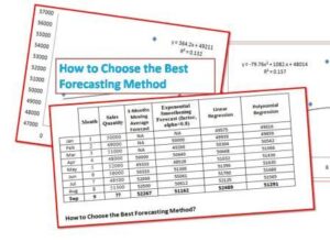
MonthSales Quantity3-Months Moving Average ForecastExponential Smoothening Forecast (factor, alpha=0.8)Linear RegressionPolynomial Regression
Jan150000NANA4957549016
Feb249000NA500004993949859
Mar351000NA492005030450542
Apr44800050000506405066851066
May55200049333485285103251430
Jun65600050333513065139651635
Jul74950052000550615176051680
Aug85130052500506125212551565
Sep9??52267511625248951291
How to Choose the Best Forecasting Method?

Now, the most important thing is to select or choose or decide the best method from the above 4 types of forecasting methods. As you can see in the above table we have mentioned the forecast value of the possible period of all 4 types of methods but even after getting the forecast value it is difficult to select the best method, so to choose the best one, we are supposed to calculate the error of each method.

MAF-Error ESF-Error LR-Error PR-Error
MonthSales Quantity3-Months Moving Average ForecastErrorSquare ErrorErrorSquare ErrorErrorSquare ErrorErrorSquare Error
Jan150000NANA NA 425180455984967783.7
Feb249000NANA -1000.001000000-939882472.4-859737812.3
Mar351000NANA 1800.003240000696484973458209617.5
Apr44800050000-2000.004000000-2640.006969600-26687117157-30669399375
May552000493332666.6771111113472.0012054784968937024570324900
Jun656000503335666.67321111114694.4022037391460421194974436519056368
Jul74950052000-2500.006250000-5561.1230926056-22605109408-21804751354
Aug85130052500-1200.001440000687.78473035.8-825679965.2-26570415.93
Sep9??52267MSE10182444 1095726745733044439703
RMSE3190.993310.182138.5282107.06

According to the above RMSE of all four forecasting methods, we found that the Polynomial Regression method is the best method in this case. So we can consider the forecast sale quantity of 9th month is 51291.

Free Templates / Formats of QM: we have published some free templates or formats related to Quality Management with manufacturing / industrial practical examples for better understanding and learning. if you have not yet read these free template articles/posts then, you could visit our “Template/Format” section. Thanks for reading…keep visiting techiequality.com

Popular Post

How to create forecast in excel | Illustration with Example

How to create forecast in excel

How to create forecast in excel | Illustration with Example:

Hi Readers! Here we are going to learn today on how to create forecast in excel. We have already published an article on basic knowledge and the selection process for best forecasting methods. As we know that forecasting is one of the common methodologies used in various types of industries for predicting the future based on the results of previous data. Here we will give more focus on the creation or preparation of the forecasting method in excel (note that, given excel process may be different from excel to excel depending on excel’s version).

Suppose a bike showroom owner would like to do the purchasing plan considering the last 4 month’s selling quantity, store constrain, Market demand, festive season, etc.  But he could not finalize the quantity. So, here we are going to do the forecast method to finalize the value (this is only the reference method and forecast value, the actual value may vary depending on various factors). Through this example, we shall learn only on how to create forecasts in excel (Some common methods only). We are going to use the excel-2007 version, the process may vary from excel version to version.

Illustration of How to create forecast in excel?

The last 9 months’ bike selling quantity is given below as;

MonthBike Selling Quantity
Jan1102
Feb2104
Mar3105
Apr4101
May599
Jun689
Jul7105
Aug8115
Sep9103
Oct10??

We have calculated a 4-Months Moving Average Forecast.

MonthBike Selling Quantity4-Months Moving Average Forecast
Jan1102NA
Feb2104NA
Mar3105NA
Apr4101NA
May599 =average(select top 4 months bike selling quantity)
Jun689 =average(104,105,101,99)
Jul7105 
Aug8115 
Sep9103 
Oct10?? 

Excel Function = Average (Select data array of 4 months)

In the above table we have mentioned the excel function. Accordingly calculated the 4-months moving average forecast value, the same table is given below. Just try to calculate the value by yourself in excel and verify the same.

MonthBike Selling Quantity4-Months Moving Average Forecast
Jan1102NA
Feb2104NA
Mar3105NA
Apr4101NA
May599103.00
Jun689102.25
Jul710598.50
Aug811598.50
Sep9103102.00
Oct10??103.00
How to create forecast in excel

How to calculate Exponential Smoothening Forecast? By considering the alpha value 0.8

Excel function, ESF of desire month = (0.8*previous month bike selling quantity + 0.2* previous month ESF)

MonthBike Selling QuantityExponential Smoothening Forecast (factor, alpha=0.8)
Jan1102NA
Feb2104102
Mar3105=(0.8*Bike selling quantity of Feb. month + 0.2*ESF of Feb. month) 
Apr4101 
May599 
Jun689 
Jul7105 
Aug8115 
Sep9103 
Oct10?? 
MonthBike Selling QuantityExponential Smoothening Forecast (factor, alpha=0.8)
Jan1102NA
Feb2104102
Mar3105104
Apr4101105
May599102
Jun689100
Jul710591
Aug8115102
Sep9103112
Oct10??105

Linear Regression Forecasting calculation in Excel:

MonthBike Selling Quantity
Jan1102
Feb2104
Mar3105
Apr4101
May599
Jun689
Jul7105
Aug8115
Sep9103
Oct10??

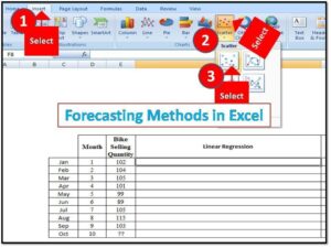
Based on the above data “month” & “bike selling quantity” plot the scatter diagram including linear regression function as per below;

How to create forecast in excel

From the Scatter diagram, you can get the function, here y=0.416*X + 100.4

By using the function we have calculated the forecast value which is given in the below table.

MonthBike Selling QuantityLinear Regression
Jan1102101
Feb2104101
Mar3105102
Apr4101102
May599102
Jun689103
Jul7105103
Aug8115104
Sep9103104
Oct10??105

Accordingly, you can calculate the Forecast value using several types of methods. But if you would like to choose or decide the best forecast value among all types then read our previous article.

Free Templates / Formats of QM: we have published some free templates or formats related to Quality Management with manufacturing / industrial practical examples for better understanding and learning. if you have not yet read these free template articles/posts then, you could visit our “Template/Format” section. Thanks for reading…keep visiting techiequality.com

Popular Post

How to make a box plot in excel | Manufacturing Example

box plot in excel

How to make a box plot in excel | Manufacturing Example:

Hi Readers! If are really searching to learn about how to make a box plot in excel then you are on the right platform. So here we are going to explain the same in detail with manufacturing or industrial examples for better understanding. And you can easily apply it in your manufacturing process to know the data symmetric. But also you can use several other tools as well. First of all, here we will learn what are box plots and their uses & interpretation.

What is Box plot?

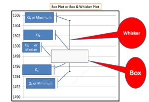
The box plot (Boxplot) or box and whisker plot is a graphical representation of numerical data spread and skewness. It helps to know whether numerical data are symmetric or not. As you know that it is also called as box and whisker plot, so the plot contains box and lines (Whiskers). It generally consists of five number summary i.e. zero quartile (Q0), First quartile (Q1), Second quartile (Q2), Third quartile (Q3), Fourth quartile (Q4).

box plot in excel

[Box plot Sample figure]

Box plot terminology:

  • Zero Quartile (Q0) or Minimum number: This is the minimum value of the data set.
  • First quartile (Q1): Lowest 25% value of the data set.
  • Second quartile (Q2) or Median: Lowest 50% value of the data set or middle value of the data set.
  • Third quartile (Q3): Lowest 75% value of the data set.
  • Fourth quartile (Q4) or Maximum number: Maximum value of the data set.
  • Inter Quartile Range (IQR): Third Quartile (Q3) – First Quartile (Q1)

How to make a box plot in excel? (Step by Step guides with manufacturing example):

Suppose a manufacturing company produces an automobile part. One day a process quality engineer has instructed to quality supervisor to record the pouring temperature reading for knowing the data symmetric by making a box plot. So the supervisor started collecting data from shift-wise and recorded the data in excel for making the boxplot. The same data are given in the below table.

Pouring Temperature in °C
1495°C
1496°C
1498°C
1499°C
1500°C
1505°C
1499°C
1497°C
Now, we have to calculate the quartile value of each quartile so the Excel function of each quartile is given below;
  • Zero Quartile (Q0) or Minimum number: =QUARTILE(array, quart)
  • First quartile (Q1): =QUARTILE(array, quart)
  • Second quartile (Q2) or Median: =QUARTILE(array, quart)
  • Third quartile (Q3): =QUARTILE(array, quart)
  • Fourth quartile (Q4) or Maximum number: =QUARTILE(array, quart)

Note, in the above excel function the “array” is the data set means for the above data table its pouring temperature data set and “quart” will be different for different quartiles. Try the given below function and calculate the each quartile value (note we have calculated all the functions and box plots by using excel 2007 version only).

Final excel function of each quartile:
Pouring Temperature in °C
1495
1496
1498
1499
1500
1505
1499
1497
  • Zero Quartile (Q0): =QUARTILE(Select pouring temperature data set,0)
  • First quartile (Q1): =QUARTILE(Select pouring temperature data set,1)
  • Second quartile (Q2) or Median: =QUARTILE(Select pouring temperature data set,2)
  • Third quartile (Q3): =QUARTILE(Select pouring temperature data set,3)
  • Fourth quartile (Q4) or Maximum number: =QUARTILE(Select pouring temperature data set,4)
Calculation of Quartiles by Using Excel Function:

Zero Quartile (Q0) or Minimum: By using the excel function given in the below figure, try to calculate the Q0 value. After applying the mentioned excel function in a given data set we found the value is 1495.

quartile calculation

First quartile (Q1): Similarly we have calculated the first quartile and the rest of the quartiles by applying the above excel function. We have mentioned the excel function in the below figure and applied the same in the pouring temperature data set and found the value is 1497.

quartile calculation
Second quartile (Q2) or Median:

Go through the below figure and calculate the second quartile value, we have found the value 1499.

quartile calculation in excel
Third quartile (Q3):
quartile calculation

Fourth quartile (Q4) or Maximum number: Apply the excel function, given in the below figure and calculate the quartile value.

quartile calculation

After applying the individual quartile’s excel function, we have summarized the all values and recorded them in the below table. Next, we are going to make a box plot in excel, so follow the below given complete guidelines or step-by-step process to make the box and whisker plot in excel.  

Q1 =1497
Min. or Q0 =1495
Q2 =1499
Max. or Q4 =1505
Q3 =1499
Upper error bar (Q4-Q3) =6
Lower error bar (Q1-Q0) =2
Step by Step Guides on How to make a box plot in excel:

Step1:

As you know that we have already calculated the quartiles values, just arrange the quartile value as per the given below figure and select the all values after that follow the step-1 to step-4 (as per the below figure).

box plot in excel

Step2: Select the option “Switch Row/Column” in excel

box plot in excel

Step3: Select the excel option as per instructions given in the below figure.

box plot in excel
Step4:

In the above process, we have plotted the box and now we have to make the whisker, so follow the below instruction as per beneath figure.

box plot in excel

Step5: Follow the below instruction

box plot in excel
Step6:

Here, we will learn the steps to make the lower whisker, so go through the below figure and follow the given instructions.

box plot in excel

Step7: similarly, we will make the upper whisker by following the below given steps

box plot in excel
Step8: Follow the steps in the below figure
box plot in excel

Step9:

box plot in excel
Conclusion and Interpretation of the above Box Plot:

As you can see the above box plot that the data are not spread in symmetric. Here we are also going to plot the histogram to compare the both boxplot and histogram to know the comparison value. You can learn more about the step-by-step guide to plotting histogram in excel with examples and also can download the histogram template or format.

Histogram:

Step1: Enter the Pouring temperature reading in excel and then calculate the interval value by using the excel function given in below figure. Next select the option “data” in excel sheet and then select “Data analysis” option and then finally select the histogram option.

box plot in excel

Step2: Select the appropriate data set as per below instruction given in figure

box plot in excel
Histogram

 Now, Histogram is ready so here we will compare the both the plot histogram vs Box plot

comparison

From both the graph we have concluded that data are not symmetrically distributed (Graph are not symmetric).

Free Templates / Formats of QM: we have published some free templates or formats related to Quality Management with manufacturing / industrial practical examples for better understanding and learning. if you have not yet read these free template articles/posts then, you could visit our “Template/Format” section. Thanks for reading…keep visiting techiequality.com

Popular Post

Attribute MSA |How to do Attribute type MSA Study| Example |Acceptance Criteria

Attribute MSA

Attribute MSA | How to do Attribute type MSA Study | Example | Acceptance Criteria

Hi readers! Today in this section we will be discussing in several topics on Attribute MSA, how to do Attribute MSA analysis, and acceptance criteria with practical industrial manufacturing examples. Measurement system analysis is one of the core AIAG tools, which is frequently used in automotive /automobile manufacturing industries to know the percentage of effectiveness, consumer risk, producer risk, etc. of those persons who are visually checking or doing inspection of parts, components, in-process products or finish products, etc.

You would love to read the below topic;

Gage R and R |How to do MSA Study | Acceptance Criteria

Attribute MSA

As you know how important visual checking /inspection is in the manufacturing industry, your wrong checking /inspection can affect the product performance or there may be a chance of rejection of the product at any stage. So it’s a very important to periodically monitor the effectiveness, miss-alarm, and false-alarm of inspectors, otherwise there will be high producer and consumer risks.

How to do Attribute type MSA Analysis?

Step-1: List out the appraisers.

Step-2: Need to have 50 references and at least 10 ‘not ok’ items.

Total references /items /components =50 nos
Ok reference =34 nos
Not OK reference =16 nos

Step-3: Note the observation of all three appraisers with 3-trials per appraiser

 Appraiser-1Appraiser-2Appraiser-3
No of opportunities150 nos150 nos150 nos
No of trial per appraiser333

Step-4: Calculate the percentage of effectiveness, misalarm and falsealarm of all individual appraisers.

Interpretation of Result and Acceptance Criteria with Example:

Suppose an organization appointed three inspectors at the final dispatch area for visual checking of the finished product. They are basically being engaged to check the visual defects. After a couple of Months Company got a customer complaint related to a visual defect and the same complaint has been analyzed by Sr. Engineer. During the validation of potential causes, he also studied the attribute type MSA of all three appraisers and he found that one of the appraiser’s percentage of miss-alarm was >5. So finally, Sr. engineer has further analyzed the root cause.  And according to the root cause action plan has been taken by him as on-job training and also he has increased the frequency of Attribute-MSA study. In this scenario, you can imagine that how important the Attribute type MSA studies are for inspectors who are doing the visual inspection.

Acceptance Criteria:

Another important part is the interpretation of the attribute type MSA study report and its decision, generally, the appraiser can be acceptable when the percentage of effectiveness is greater than or equal to 90, the miss-alarm less than or equal to 2, False-alarm less than or equal to 5. And also appraiser can be marginally acceptable but may need improvement when percentage of effectiveness greater than or equal 80, miss-alarm less than or equal to 5, False-alarm less than or equal to 10.

Similarly, the appraiser can be unacceptable when the percentage of effectiveness is less than 80, the miss-alarm greater than 5, False-alarm greater than 10.

The general thumb rule of kappa is that, if the kappa value > (greater than) 0.75 then it indicates good agreement (but note one thing that the maximum kappa value will be 1 and it indicates excellent agreement). and similarly, the kappa value < (less than) indicates the poor agreement.

Please note that all the above acceptance criteria are the general thumb rule.

learn more about multiple types of questions and answers of MSA. then click here.

Free Templates / Formats of QM: we have published some free templates or formats related to Quality Management with manufacturing / industrial practical examples for better understanding and learning. if you have not yet read these free template articles/posts then, you could visit our “Template/Format” section. Thanks for reading…keep visiting techiequality.com

Useful Post:

How to Plot Scatter Diagram in Excel? |Guides with example | Interpretation

Scatter Diagram Template |Industrial Example |Download Excel Format

How to do data analysis by excel sheet? Step by step guides

Types of Fishbone Diagram |Dispersion Analysis |Enumeration |Process Classification

More on TECHIEQUALITY